A bulk of the research performed for the Drone Estimation Lab focuses on the Extended Kalman Filter (EKF) state estimator and error ellipsoid generation based on covariance matrices. The state estimator is imperative for the combination and utilization of sensor data for the drone, and the error ellipsoid generation will be used in the future for collision avoidance during GPS denied flight.
Extended Kalman Filter
A Kalman Filter is a filter that uses a less-than-perfect dynamic model and noisy measurement inputs to provide very accurate state estimations for a system. However, this filter will only work for linear systems. An Extended Kalman Filter (EKF) is a type of Kalman Filter that is used for state estimation in non-linear systems. It is an extension of the standard Kalman Filter, able to handle non-linear systems by approximating the non-linear function with a first-order Taylor series expansion. The EKF works by using a state transition function and a measurement function to estimate the state of a system. The state transition function describes how the state of the system changes over time, while the measurement function describes how measurements of the system are related to its state.
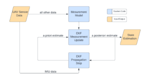
This diagram describes DEL’s EKF. Gathered sensor data from the UAV (input) is sent to the EKF for propagation. After an a priori estimate is made it is compared to new data gathered by the sensors. An a posteriori estimate is then used as the state estimation (output) and also sent back to the EKF for the next propagation step. This cycle continues on the realtime data.
The state usually consists of the drone position, velocity, and pose parameters stacked in a vector. The Kalman Filter needs a state propagation equation, which describes how the state would evolve in a perfectly deterministic environment. Instead of modeling the complex drone dynamics we adopt a model replacement approach, propagating the IMU’s state as a proxy for the drone’s state. Due to the high IMU data rate we can propagate the IMU state in the propagation step by simple euler integration.
Error Ellipsoid
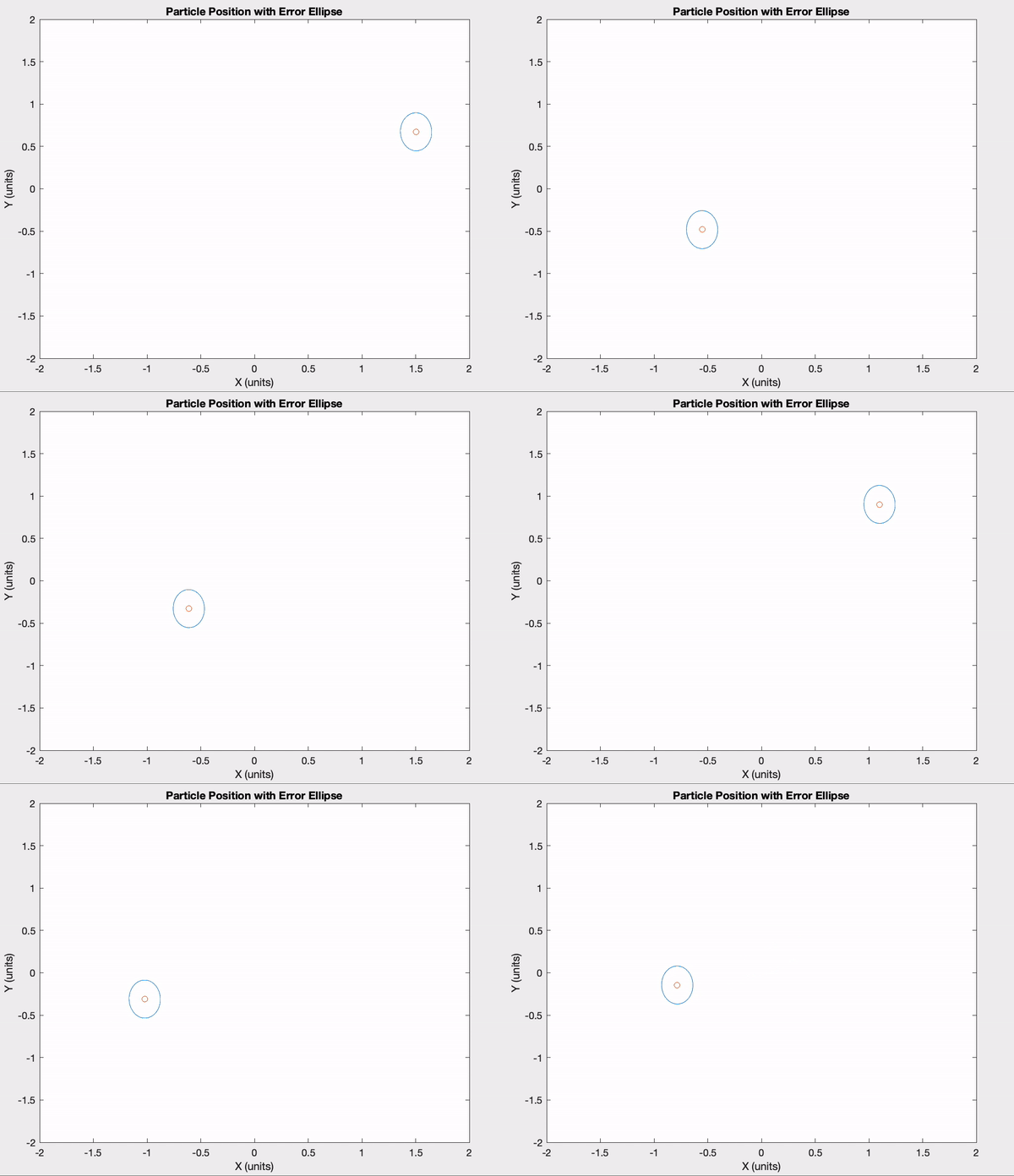
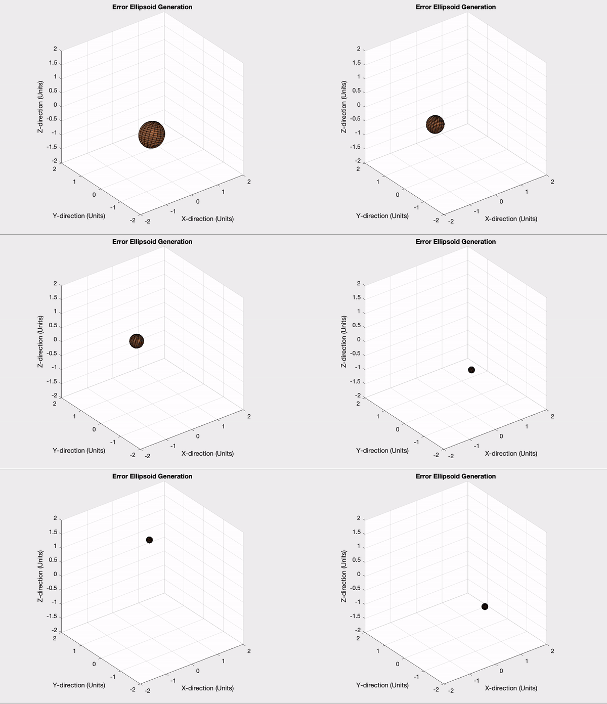
The ultimate error visualization method to be used in this project is the three dimensional error ellipsoid. However, the effort necessary to develop an algorithm and graphical visualization for a 3D error ellipsoid of a drone is quite excessive for an initial demonstration. Because of this, early work for this project involved creating and visualizing 2D error ellipses instead, an example of which is shown in the video below titled “Particle Position with Error Ellipse”. This creates an error ellipse based on the movement of a particle through 2D space. After the completion of this model, the 2D model was extended into 3D space by adding an additional term to the dynamics model. This model is visualized in the below video titled “Error Ellipsoid Generation”.
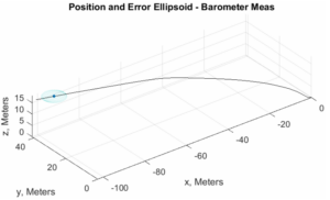
The error ellipsoid is to be shown as the visualization of a 3D Gaussian model of a certain probability area. The diagram below depicts the current MATLAB workflow to plot the drone error ellipsoid using a given covariance matrix.
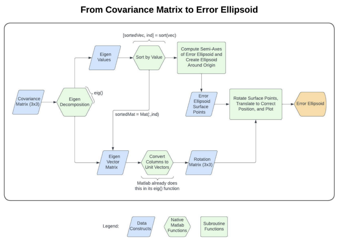
Starting with the covariance matrix that we get from our data, the eigen decomposition finds the eigenvalues and eigenvectors, which will describe the size and orientation of the error ellipsoid: the eigenvalues are used to compute the magnitudes of the semi-axes, and the eigenvectors are used to create the rotation matrix, which describes the orientation of the semi-axes derived from the eigenvalues.
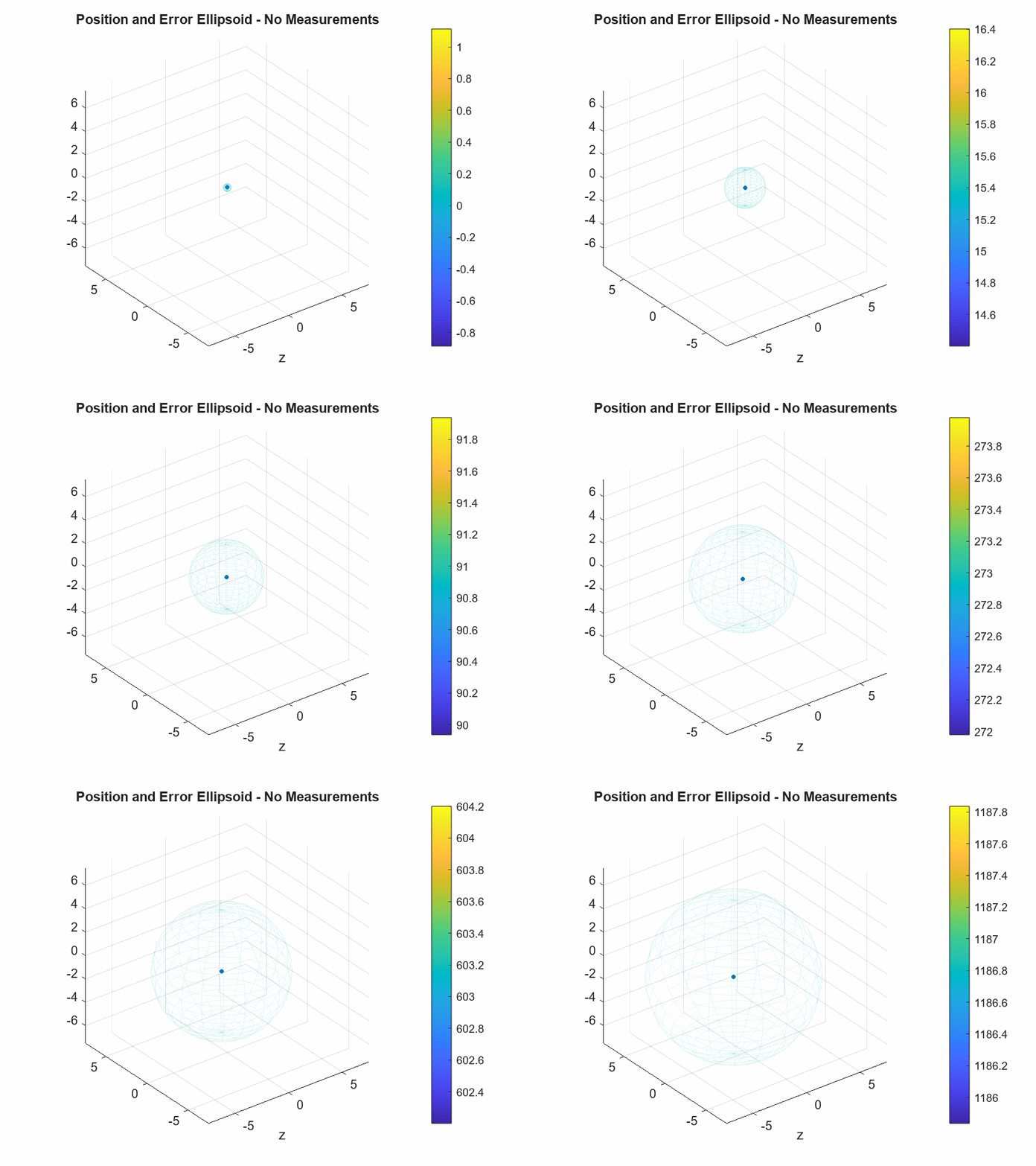
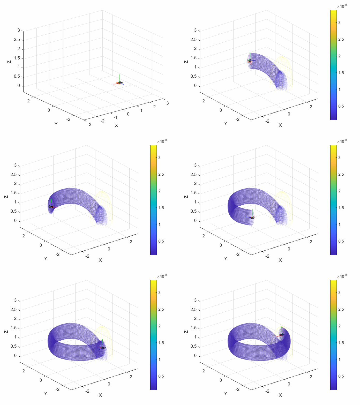
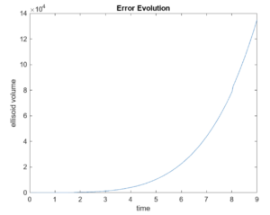
If the measurement update does not introduce new data in the Kalman filter process, then the prediction step is essentially integrating the IMU measurements, and the noise and bias associated with them. This causes the error ellipsoid volume to grow exponentially, as seen in the graph below.
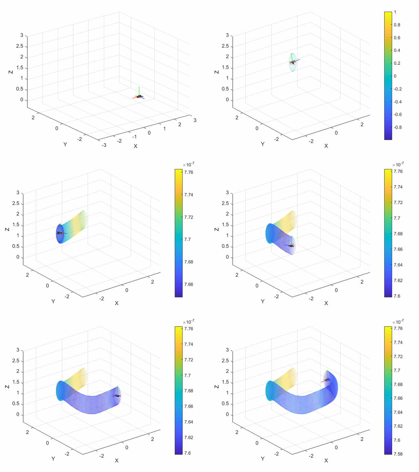
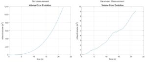
With the inclusion of even one additional sensor into the measurement model, the error ellipsoid volume is greatly reduced relative to the system with no new data. This is observed below in the error ellipsoid volume over time graphs below for the EKF without a measurement model and for the EKF including barometer measurement.
The animation below shows the actual position and error ellipsoid for both the no-measurement model and the model using the barometer.
As seen in the animation, the reduction in ellipsoid volume is due to the reduction of the vertical semi-axis of the error ellipsoid. The inclusion of the barometer measurements improved the estimation of the altitude. With the inclusion of more sensors for other state variables, the error ellipsoid volume should continue to also improve and decrease in volume.
3D MATLAB Drone Simulation
Now that a 3D error ellipsoid was successfully plotted for an arbitrary potential field the next step is applying the knowledge found from the previous models to a simulated drone model with actual dynamics representative of what we will see going forward in the project. With that in mind a simulation of a drone based on a model-based approach, developed in another class, is adapted to output the error covariance matrix found during the Kalman filter implementation in said simulation. The three sensors used in this simulation are a camera, a MEMS IMU, and a CD-GNSS. The camera is modeled with a pinhole camera model and uses known points in its field of view to solve Wahba’s pose estimation problem. The IMU is modeled with a bias for both the accelerometer and the gyroscope. There are two CD-GNSS receivers mounted on the drone which provide very accurate measurements. All sensors are modeled with gaussian noise. The simulated trajectory is a circular flight around the origin at a height of one, and the drone is controlled by the implementation of a PD controller. The resulting error ellipsoid is plotted by taking the covariance matrix, found by running the simulated sensor measurements through the Kalman filter, reducing it to a 3×3 position error covariance matrix, and performing the operations detailed in the above sections. The below gifs showcase the drone’s behavior utilizing different gains along with the corresponding error ellipsoid.
Testing – SITL and HWITL Results
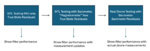
SITL to Real Drone Testing Pipeline
The testing pipeline started out with Software-In-The-Loop (SITL) with just the propagation step turned on using the IMU accelerometer and rate gyroscope data. We ran the simulation for multiple different trajectories: linear trajectories along X,Y, and Z axes, and then a circular trajectory.
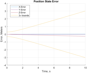
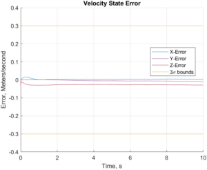
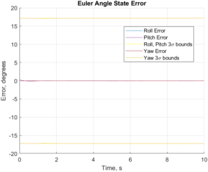

Linear X-Direction SITL Trajectory Performance with only IMU
As seen in the figures above, the linear trajectory performed well even with just the IMU data, granted that the test was over just a 10 second period.
The circular trajectory, however, struggled a bit more with the state estimation.
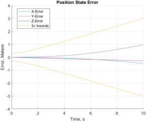
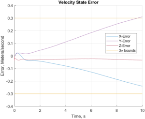
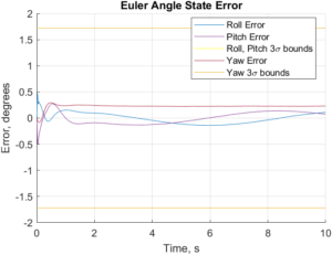
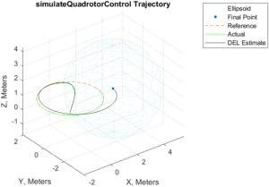
Circular SITL Trajectory Performance with only IMU
The EKF notably struggles a lot more with this circular trajectory, with the position and velocity error growing as time passes. This error stays relatively within bounds for the 10 second period, but as the figures show, at least the velocity error is already crossing or about to cross the bounds at around the end of this time period. Additionally, the yaw error seems to indicate some sort of bias, although this may be an issue within how we are simulating things or within the code.
Nevertheless, this first stage showed us two things – that our filter was working relatively as expected and how the filter was performing without any measurement updates in a simulated environment.
Next, the SITL test is updated to include simulated barometer and magnetometer measurements, which allowed us to see how including these measurement updates affected filter performance.
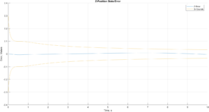
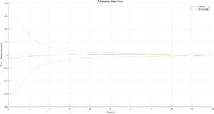
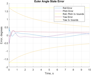
Circular SITL Trajectory Performance Changes with Barometer and Magnetometer Updates
The changes we saw were in the above figures – the performance and confidence level of the z-position and z-velocity improved thanks to the barometer, and the confidence bounds of the yaw also get narrower with the updates of the magnetometer. It is of note that the z-velocity error does cross out of the confidence bounds near the end of the testing period, though.
Lastly, we gathered real drone IMU, barometer, and magnetometer data to test the SITL with. This stage has only currently been done in post-processing, but eventually the code will be converted from MATLAB to Python and running onboard the drone for true real-time performance. During the 2024 Spring semester, we unfortunately could not get the GPS running in time, so residuals between the estimate and the barometer altitude are used here instead. Preferably, a comparison against GPS as the “truth” data will be done in the future.
We started out with a stationary drone dataset for calibration purposes and for a preliminary run of the filter.

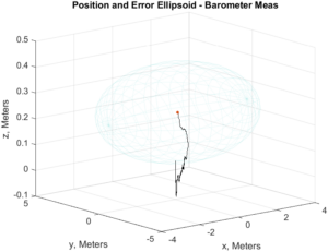
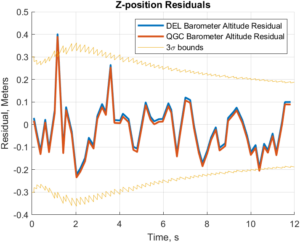
Stationary Drone – Path w/ Ellipsoid, Path w/ End Ellipsoid (stretched), Z-position Residuals
It doesn’t do too badly, but we can observe by the end of our data collection period of 12 seconds that the path is definitely drifting away from the origin, where it should have stayed.
Our next test was with a horizontal run.

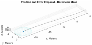
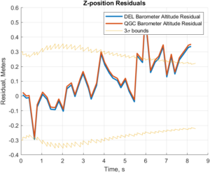
Horizontal Path w/ Ellipsoid (Left 2) and Z-position Residuals (Right)
Our EKF was able to get the general direction of movement. However, the distance traveled seemed to be greatly inflated, as the original drone had likely only traveled about 3 meters. Additionally, we can see that the error seems to drift out of confidence bounds pretty early at 5 minutes for the z-position.


Vertical Path w/ Ellipsoid (Left 2) and Z-position Residuals (Right)
Again, the horizontal position seems to be thrown very off, which may be due to some other unaccounted factor within code or calibration. However, the vertical state estimation performs better this time, reaching an estimated 18 meters of vertical distance traveled. The z-position residuals also notably stay relatively within confidence bounds before drifting off after about 10 seconds.
Block Diagram
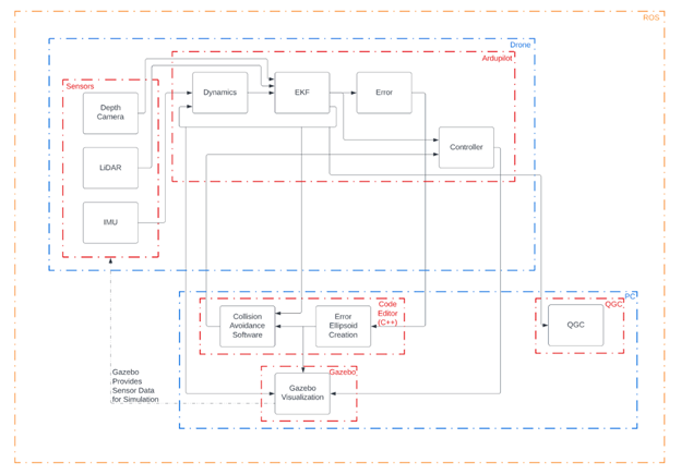
Depth Camera:
A depth camera is often a stereo camera created with the ability to sense depth in an environment. This is useful as the front facing camera on a drone because it helps the drone track how close obstacles are to it.
LiDAR:
LiDAR is a system that uses light pulses to map out an environment. The pulse emitter shoots lasers of light out that reflect back to the receiver. Using the time it took for the light to bounce back, the system generates a 2D or 3D map/representation of the environment.
IMU:
The IMU, or Inertial Measurement Unit, is one of the main sensors that will be used on the drone. The IMU measures body forces and angular rates using accelerometers and gyroscopes. IMU’s are often used in aircraft and unmanned aerial vehicles like drones. The IMU will help provide the angular rates of the drone, which are crucial in determining the states of the drone. The IMU can also provide acceleration information via the accelerometers, which can be used to find velocity and position of the drone, which are other key states of the drone.
Dynamics:
Understanding quadcopter dynamics is essential to predicting the next state in the Extended Kalman Filter. Each opposing quadrotor blade spins in the same direction and every neighboring blade spins in the opposite direction. The symmetric placement of rotors and strategically chosen spin direction let the quadcopter be able to produce, within hardware capability, an arbitrary combination of attitude and thrust magnitude. It cannot however produce an arbitrary thrust vector and attitude vector, as the equations are coupled.
EKF:
The Extended Kalman Filter is a state estimator that combines sensor measurements, the stochastic properties of each sensor and the dynamics of the quadcopter to stochastically determine the most likely position at each time new measurement data is available. The EKF linearizes the non-linear dynamics of the quadcopter to analyse local behavior, which makes it computationally light compared to other non-linear filters.
Error:
The error outputted from the Extended Kalman Filter block is in the form of the covariance matrix. The covariance matrix in this context is a square matrix that contains values that correlate the possible error in each state based on each of the other states. This covariance matrix can be used by the error ellipsoid software to create a visual representation of the error in the form of the error ellipsoid.
Sensor uncertainty related to process noise and bias are also accounted for in the form of covariance matrices. Generally, the process noise covariance matrix and bias covariance matrix can be found using sensor specifications and the intervals of sensor measurement.
Controller:
A dynamics controller is a system that uses feedback control to manipulate the behavior of a dynamic system in order to achieve a desired outcome. It analyzes the state of the system and compares it to a desired state, then applies control inputs to steer the system towards the desired state. This type of controller is commonly used in engineering fields such as robotics, aerospace, and mechanical systems to stabilize or optimize the behavior of dynamic systems.
QGroundControl (QGC):
QGroundControl is an open-source software application that provides a user-friendly interface for configuring and controlling autonomous vehicles. It supports a variety of unmanned aerial vehicles (UAVs) and ground vehicles, and allows users to plan and execute autonomous missions, view real-time telemetry data, and monitor vehicle status. QGroundControl also includes features for manual control, such as joystick support and video streaming.
Collision Avoidance:
A collision avoidance algorithm is required for every autonomous vehicle to determine a safe trajectory for navigation. The software algorithm needs to be able to process the sensor data and predict the quadcopter’s current trajectory to determine possible adjustments that may need to be made to avoid collisions with objects. This algorithm would also need to be integrated with the flight controller to ensure real-time adjustments to the quadcopter’s flight path. The collision avoidance algorithm would be one of the final steps to flying a quadcopter autonomously in an urban environment.
Error Ellipsoid:
Due to inevitable errors in sensor measurements and inaccuracies in drone dynamics models, the exact state of a drone cannot ever be computed. The error ellipsoid is a visual representation of this state uncertainty for the drone’s position. Error ellipsoids have confidence intervals, which indicate the probability of the drone’s position being within the bounds of the ellipsoid. For our latest simulations, the error ellipsoids have 97.1% confidence, meaning that the drone’s position has a 97.1% chance of being within the ellipsoid’s bounds. We generate error ellipsoids using the covariance matrix of the drone’s state, which is an output of the EKF. Since the drone’s state changes over time, the covariance matrix, and in turn the error ellipsoid, change as well.
Data Visualization and Gazebo
Gazebo Visualization:
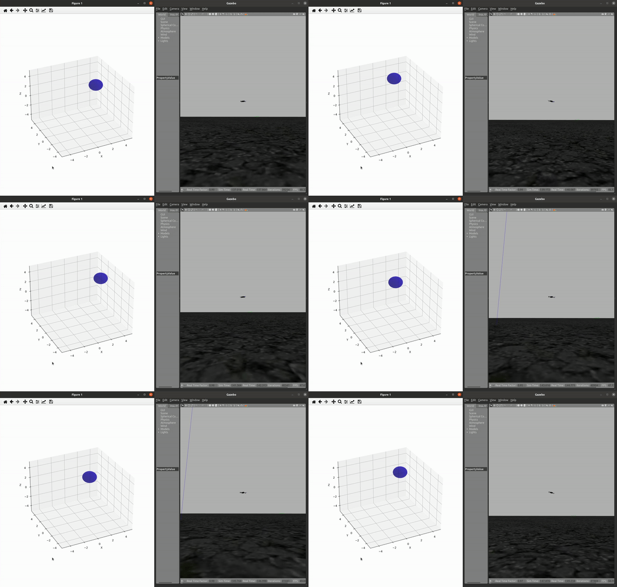
Gazebo is a popular open-source software tool used to visualize and simulate a variety of robotic systems. Initially, this software will be used to visualize the simulation of a quadcopter and provide sensor information for testing and evaluating different control algorithms and strategies on a quadcopter. This software-in-the-loop (SITL) implementation is currently being developed, with a connection to QGroundControl while using a real hardware flight controller. Eventually, the use of Gazebo will shift more towards visualizing and analyzing real-world flight data captured from a physical quadcopter, allowing for a more detailed and interactive view of the quadcopter and a generated error ellipsoid. The below images show an example of the current SITL gazebo simulation with a generic quadcopter frame (left) and a diagram of the mavros connections (right), including the connection to our own script which is able to pull pose information from the drone in real time.
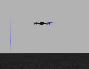
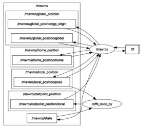
As of December 2023, the lab now has working real-time ellipsoid visualization capability, both in SITL and HITL simulation environments. The ellipsoid does not carry any estimation information yet, but the position of the ellipsoid updates in real time to reflect the position of either the simulated drone (in SITL) or the hardware flight controller (in HITL). The script in written in python using the matplotlib library and already contains inputs for the EKF outputs to feed into, which will make integration with the EKF more seamless. The below gif shows the visualization in SITL, and the video provides an overview of the pipeline for SITL and HITL scenarios, as well as a demonstration.
