Convex domains

December 2, 2024, Filed Under: Convex domains, Demos

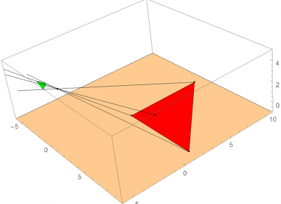
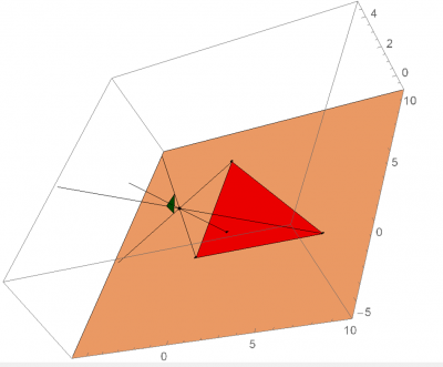
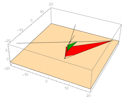
The final version of the rounding algorithm is available below; feel free to manipulate the number of vertices, the inclusion and position of the bug, and the orientation of the vertices. The roundness ratio and the matrix which records the accumulated transformations on this image are in the upper left. The bug itself is displayed as a white dot inside the image, and the center is displayed as the smaller red dot. One special case to note is that due to the random generation of the polygon, there are times when the bug will spawn outside of the image. When this occurs, the program will force all vertices on the far side of the image to wrap around the bug before beginning to center the bug. Thus, the resulting image’s roundness will still reach at least 0.5 as stated above as long as it is still convex; however, compared to the original polygon, the image will be flipped inside out.

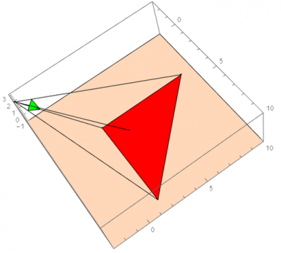
Figure 1: special case where bug generates outside polygon

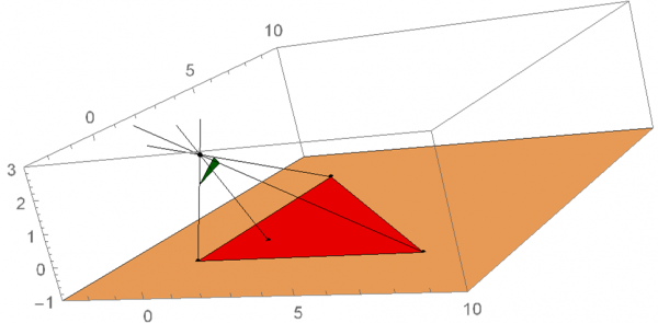
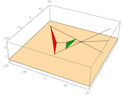
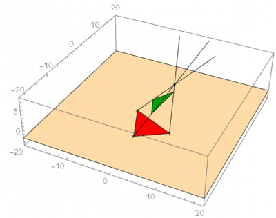
Figure 2: with more vertices, the minimum roundness can still be reached by using the bug to force multiple vertices together

December 2, 2024, Filed Under: Convex domains, Rounding Algorithm

Rounding Algorithm

Convex domains in projective geometry

Our next discussion covered how to determine the optimal roundness of a particular shape or object’s image. We described optimal roundness as the minimization of the ratio between the radius of the circumscribed and inscribed circles of a polygon. We then aimed to measure how round a convex polygon’s image could be made using particular types of transformations.

Version 1: Affine Transformations

Our first attempt dealt with solely affine transformations, specifically rotating or scaling along an axis. Testing randomly generated convex polygons, we created a program which repeated this affine optimization procedure until no further iterations improved the image’s roundness:

Locate the longest axis of the image
Rotate the image such that the longest axis was parallel to the x axis
Scale the image down by some fixed constant along its longest axis
Rotate the image back to its original orientation

Version 2: Affine and Projective Transformations with Bug

The second version of the program combined affine and projective transformations in sequence, with a pair of affine and then projective transformations constituting a single step in the iterative process. The projective optimization was nearly identical to the affine optimization, except with a projective transformation (incrementing elements i or j in the projective linear transform matrix) replacing step 3 in the procedure listed above. For visual aid, we displayed the axes of optimization using lines colored red (for affine transformations) and blue (for projective transforms between the bug and the “center” of the polygon).

We also combined roundness optimization with a similar concept of the “bug” from the previous experiment; we determined how to increase the roundness of the projection in such a way that the image of a “bug” placed on its surface appeared to move towards the center of the projection. The center of the projection could be defined as any arbitrary point within the polygon, and the experiment still functions as intended (we experimented with the polygon’s center of mass, the inscribed circle’s center, and the average between the circumcircle’s center and the inscribed circle’s center). We selected the polygon’s “center” to be the center of its circumcircle; we found that this definition resulted in more direct movement of the bug toward the center. In this context, the “longest axis” referred to by the optimization procedure is locked in as the distance between the center and the bug.

Testing this program with convex polygons of up to one hundred vertices, we can observe consistent results regarding the image’s lower bound of roundness. With the added constraint of the bug, the minimum roundness is about 0.5 (comparative to that of an equilateral triangle, seen in figure A). Without the bug, the minimum roundness is about 0.7 (comparative to that of a trapezoid, seen in figure B). These convergences are a result of successive projective transforms which appear to “squish” all but two or three vertices into one vertex, so that the final image appears to have only three or four vertices (depending on if the bug is present or not). Polygons with greater number of vertices tend to generate with higher roundness, as they are convex. In these cases, if the bug is present, one can move the bug far from the center to observe how the projective transformations compress vertices on the opposite side together.

Below: typical performance of final version of algorithm; note that projective transforms are generally used less often than affine transformations

December 2, 2024, Filed Under: Bugged Triangle, Convex domains

Bugged Triangle

Convex domains in projective geometry

After this initial overview of triangle projection, we added a “bug” on the triangle: a fixed point around the middle of the triangle, which was projected as a singular point within the (now translucent) triangle’s shadow. We studied how to reposition the triangle such that the bug’s shadow moved but the triangle’s shadow remained the same. For a fixed distance between the center of the triangle and the observation plane, the four solutions for a projected equilateral triangle are displayed below.

Below: solutions to bug problem for a fixed triangle and distance between the triangle and observation plane

December 2, 2024, Filed Under: Convex domains, Projecting Triangles

Projecting Triangles

Convex domains in projective geometry

This project began with an observational experiment which expanded into projective space as we learned more about projective linear transformations. We first set out to determine the types of triangles which could be projected by a flat, equilateral triangle given a movable point source. As seen below, we could orient the point source in any relation to the triangle, and we observed the resulting projections on some arbitrary plane (in this example, the z = 0 plane). Depending on how we rotated the triangle and positioned the point source, the size and shape of the shadow changed. We repeated this experiment with various kinds of triangles, and found that any type of triangle could be projected regardless of the characteristics of the original triangle. In other words, nothing about the size or side lengths of a triangle could be determined by simply observing its shadow.

We calculated the orientation of the triangle based on nine parameters: three parameters corresponding to the position of the point source, and two parameters for each of the vertices of the triangle. We described the vertices of the projection using lines extending from the point source through the vertices of the triangle and intersecting with the observation plane.

Below: various triangles could be projected (in red) with a constant original triangle (in green).