Hyperelastic Material Analysis with Los Alamos Laboratory

I participated in a Research Experience for Undergraduates with Los Alamos National Laboratory and the Texas A&M Department of Material Science and Engineering in the summer of 2021. The video below is my final presentation of the internship’s work.

In this internship, I was responsible for providing estimation of material parameters and feedback on the manufacturing process of an undisclosed rubber. The diagram below lists the process, which leaned heavily on curve fitting, continuum mechanics, and statistical analysis.

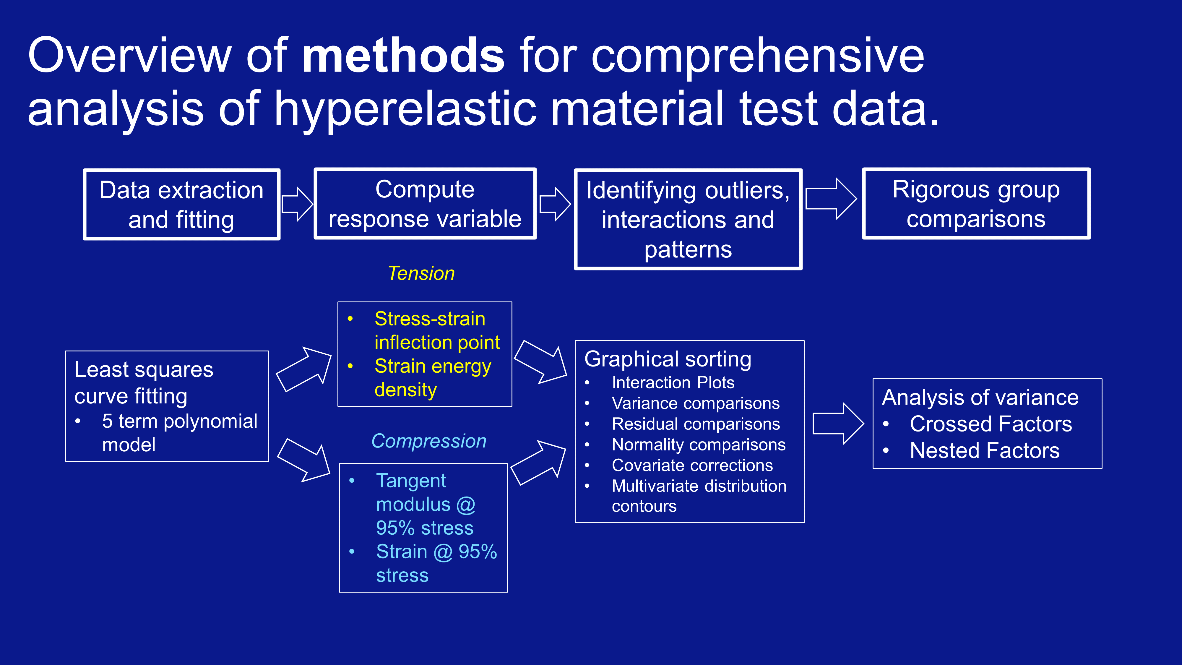
The analysis was all done in Matlab. I fitted polynomials based on continuum mechanics to the test data, the fits were excellent. From these fits, I could extract estimates of material properties despite the nonlinear stress strain relationship.

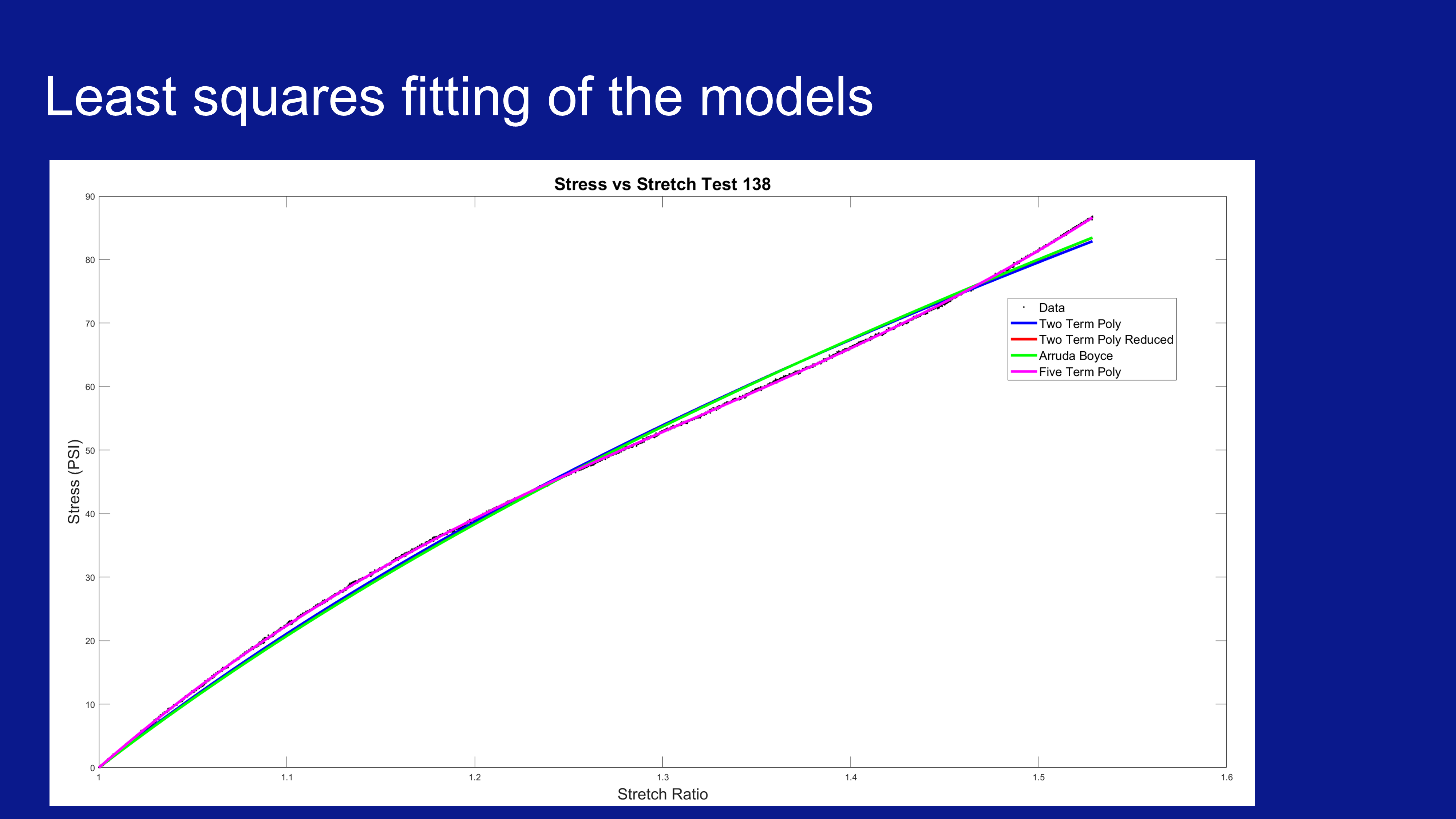
Test data along with multiple fitted hyperelastic models.

The code below parses through the test data, fits curves to it and saves the coefficients and material estimate properties for comparison.

filePath;
load('file_listTension.mat'); 
load('tabulatedData.mat');
min_upper_bound = 100;
for i = 2: length(file_list)
    load(file_list(i));
    
    if max(record.data.x) < min_upper_bound 
        min_upper_bound = max(record.data.x);
    end
    
    analysis.poly5eq = @(c, x)c(1).*(x.*2.0-1.0./x.^2.*2.0)-c(2).*(1.0./x.^3.*2.0-2.0)+c(4).*(x.*2.0-1.0./x.^2.*2.0).*(x.*2.0+1.0./x.^2-3.0)-c(5).*(1.0./x.^3.*2.0-2.0).*(x.*2.0+1.0./x.^2-3.0).*2.0+c(3).*(x.*2.0-1.0./x.^2.*2.0).*(2.0./x+x.^2-3.0).*2.0-c(4).*(1.0./x.^3.*2.0-2.0).*(2.0./x+x.^2-3.0);
    
    [analysis.poly5coff, organizedData(i-1).resNormPoly5] = lsqcurvefit(analysis.poly5eq, [79.5011  -39.1285  -69.9408  256.7353 -250.76], record.data.x', record.data.y');
    
    [organizedData(i-1).c10Poly, organizedData(i-1).c01Poly, organizedData(i-1).c20Poly, organizedData(i-1).c11Poly, organizedData(i-1).c02Poly] = deal(analysis.poly5coff(1), analysis.poly5coff(2), analysis.poly5coff(3), analysis.poly5coff(4), analysis.poly5coff(5));
    
    syms x;
    
    poi_set = solve(diff(analysis.poly5eq(analysis.poly5coff, x),2) == 0, x);
    
    [organizedData(i-1).poly5POIX, analysis.poly5poiX] = deal(double(poi_set((isAlways(poi_set >= 1)) & (isAlways(poi_set <= max(record.data.x)))))); % Extract the root which is in the data's domain
    [organizedData(i-1).poly5POIY, analysis.poly5poiY] = deal(double(analysis.poly5eq(analysis.poly5coff, organizedData(i-1).poly5POIX)));
    
    save(file_list(i), 'analysis', '-append');
    
end

%After solving for the lowest maximum strain, integrate the fitted curve
%from 1 that value
for i = 2: length(file_list)
    
    load(file_list(i));
    syms lambda
    [analysis.strainEnergy, organizedData(i-1).strainEnergy] = deal(double(int(analysis.poly5eq(analysis.poly5coff, lambda), lambda, 1, min_upper_bound))); %Analytically from the fit
    
end

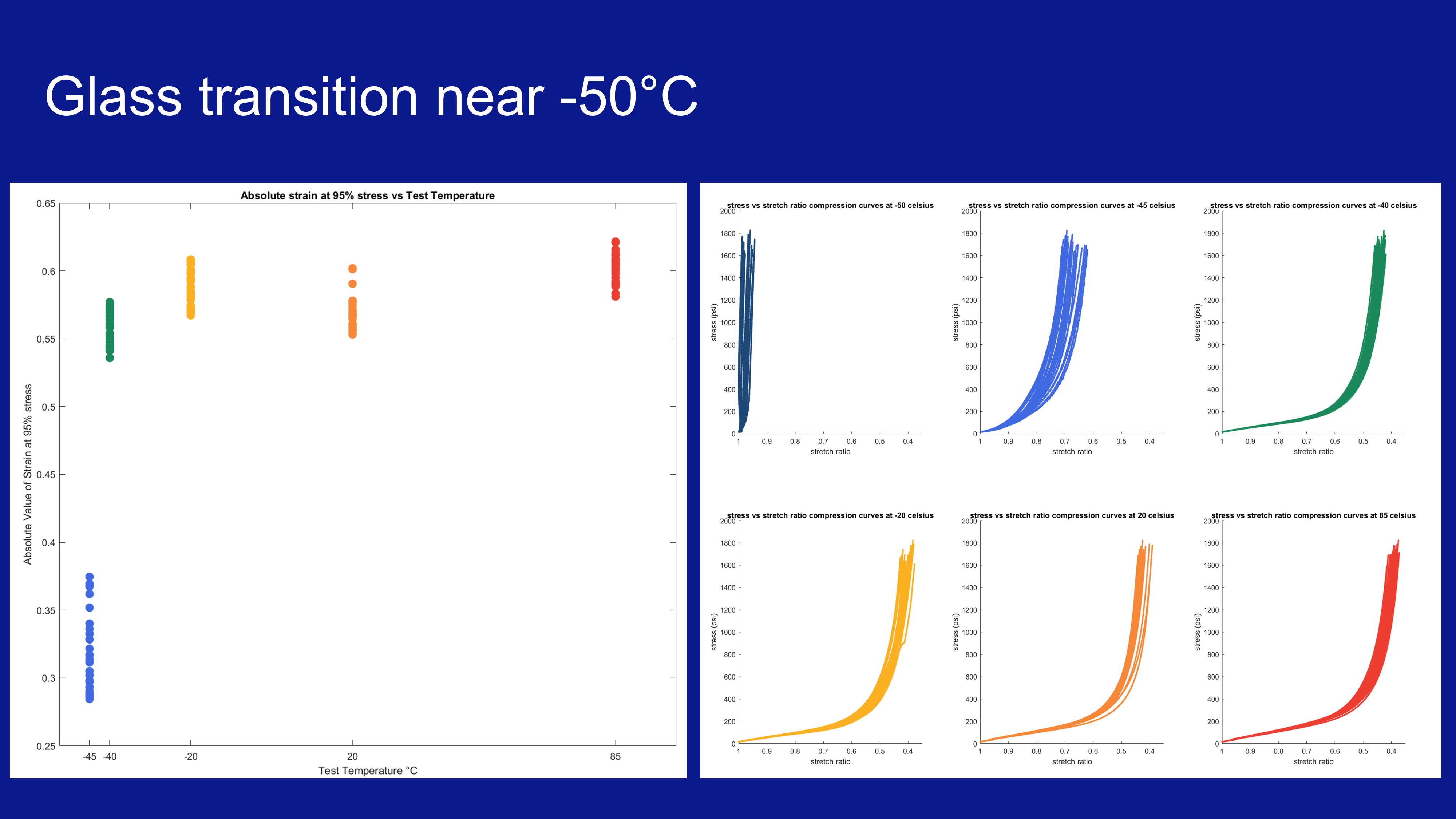
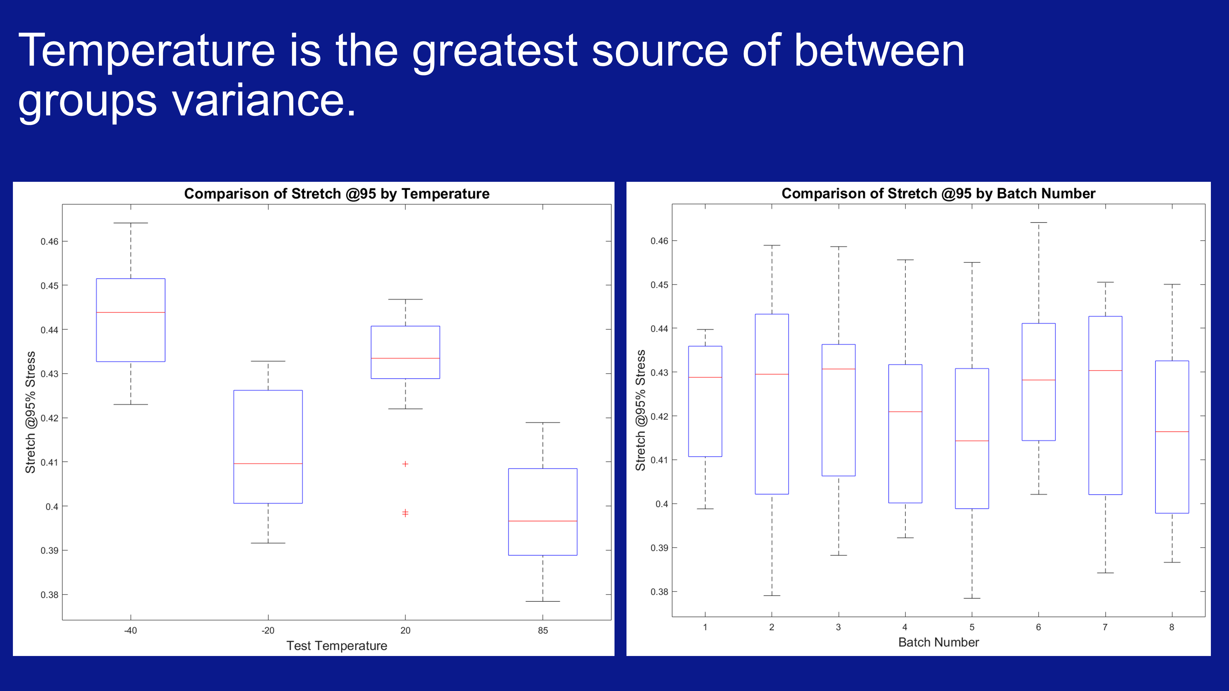
save('tabulatedData', 'organizedData');

After estimating material properties from these tests, they could be more powerfully compared with statistical methods to find conditions which had the greatest effects on these properties. The most significant of this was the test temperature. The plots below show this not only visually but also numerically.

Strain near max test stress comparison across test temperatures.

Analysis of variance with test temperature and material batch number.

I was ultimately able to make estimates of these material properties and how the testing regime affected them, including predictions that drew on established research at the microstructure scale of hyperelastic materials. In the slide below I made an estimate about chain straightening on the microscale that creates a foundation for future investigation.