For research involving a numeric variable of interest, descriptive statistics of the variable are frequently presented at the beginning of a journal article or other report of the results. Describing a variable’s distribution provides readers a context for further statistical analysis.
When describing a numeric variable, it is important to include information about the following:
- Shape – what is the shape of the distribution?
- Center – what is an “average” value?
- Spread – how far away from the center do values tend to fall?
- Unique features – are there any outliers?
The appropriate measure of center and spread used to describe a variable depends on the shape of the distribution. Therefore, it is important to first visualize the variable’s distribution by creating a histogram.
If the distribution is symmetric, then the mean and standard deviation should be used to describe the center and spread. If the distribution is skewed, then the median and IQR (inter-quartile range) should be used. It is also common to include the 5-number summary (minimum value, first quartile, median, third quartile, and maximum value) to describe a distribution. See the equations below to calculate each of these summary statistics.
Relevant Equations:
Let x = data value, n = sample size
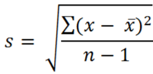
Mean:
![]()
Sample Standard Deviation:
s2 = sample variance
Median: Center point of data when sorted in order from least to greatest. If there is no exact center value (if you have an even number of responses), take the average of the two center values.
Interquartile Range: IQR = Q3 – Q1
Q1, the first quartile, is the median of the lower half of the sorted data (25% of the values fall below Q1).
Q3, the third quartile, is the median of the upper half of the sorted data (75% of the values fall below Q3).
Typically, when calculating Q1 and Q3, the median of the data is not included. However, some textbooks do say to include the median in each half when calculating Q1 and Q3.
Examples:
Normally distributed data:
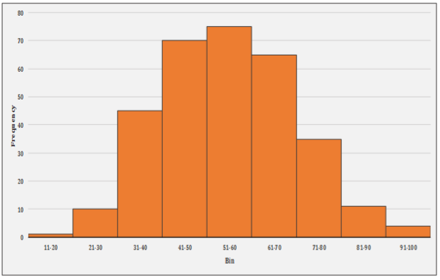
The shape of the distribution is symmetrical and approximately normal. The minimum for the data is 13 and the maximum is 100. The mean of the distribution is 54.97 and the standard deviation is 15.44. The data does not appear to have any outliers.
Skewed data:
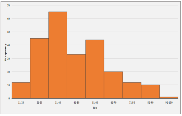
The shape of the distribution is skewed to the right. The minimum for the data is 11 and the maximum is 92. The median of the distribution is 40 and the interquartile range is 25. The data does not appear to have any outliers.
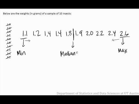
Example 1: Hand calculation
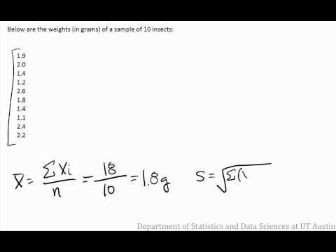
These videos describe calculating descriptive statistics by hand for the weights of a sample of 10 insects.
5-number summary (includes median and quartile calculations)

Mean and standard deviation
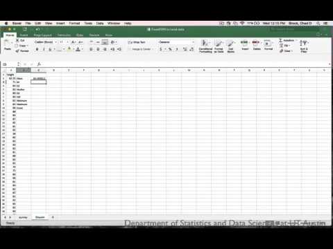
Example 2: Performing analysis in Excel 2016 on
In this tutorial you will learn how to calculate the mean, standard deviation, and 5-number summary for heights.
PDF directions corresponding to video
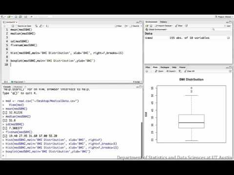
Example 3: Performing analysis in RStudio
This video covers calculating the mean, standard deviation, median, and IQR of BMI for a sample of patients.
Dataset used in video
R script file used in video