A one-sample t-test can be run on sample data from a normally distributed variable to test if a population mean μ is equal to a specific claimed value. For example, suppose you asked a sample of students how many hours of sleep they get on a typical week night. You could then test whether or not, on average, the population of students get eight hours of sleep with this method. The test statistic, t, is calculated by subtracting the claimed population mean from the sample mean and dividing by the [tooltip tip=”equal to the sample standard deviation divided by the square-root of the sample size”]estimated standard error[/tooltip].
Hypotheses:
Ho: The population mean equals the claimed value, or μ = μo
HA: The population mean does not equal the claimed value, or μ ≠ μo
The estimated standard error of the mean:

The test statistic (where μo is the claimed value from the null hypothesis):

For more information on how to calculate the sample mean and standard deviation, see this page.
If the sample mean is far enough away from the claimed mean, then the test statistic t will be large enough to produce a p-value < α and there will be evidence against the null hypothesis.
Assumptions:
- Random samples
- Independent observations
- The population is normally distributed.
If the third assumption is violated, an alternative test is the Sign Test, which tests if the [tooltip tip=”the midpoint of a distribution, where 50% of the values fall below it and 50% fall above it”]median[/tooltip] of a variable differs from a claimed value.
Example 1: Hand calculation video
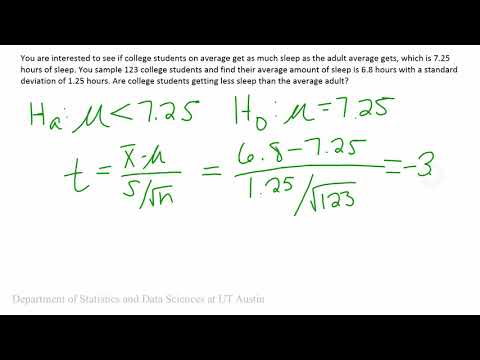
This video analyzes if college students get 7.25 hours of sleep, on average, based on a sample of students:


Sample conclusion: After completing a one-sample t-test with t(df=122)= -3.99, which was more extreme than our critical value of -1.66, we find evidence to suggest that the mean number of hours of sleep that college students get is less than 7.25 hours.
Example 2: How to run in Excel 2016 on
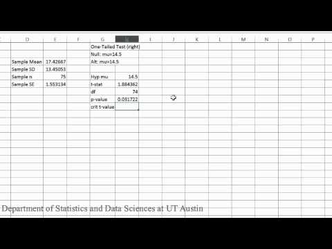
In this tutorial you will learn how to test the mean amount of time students spend on the phone in several different scenarios.
Dataset used in video
PDF directions corresponding to video


Sample conclusion (right tailed test): After completing a one-sample t-test with t(df=74)=1.88, p=0.03, we found evidence that students do spend more than 14.5 hours on their phone each week, on average.
Example 3: How to run in RStudio
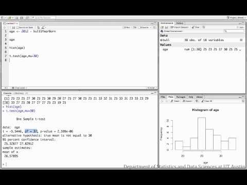
The dataset used in this video is a collection of variables for 38 professional bull riders, including their ranking in the professional league, how many events they’ve competed in, and their respective birth years. This video shows how to test the hypothesis that the mean age of the bull riders is 30 years.
Dataset used in video
R script file used in video


Sample conclusion: After completing a one-sample t-test with t(df=37)=-5.54, p<0.001, we have evidence that the mean age of professional bull riders is not 30 years.
