A multi-factor ANOVA or general linear model can be run to determine if more than one numeric or categorical predictor explains variation in a numeric outcome. A multi-factor ANOVA is similar to a one-way ANOVA in that an F-statistic is calculated to measure the amount of variation accounted for by each predictor relative to the left-over error variance. A general linear model, also referred to as a multiple regression model, produces a t-statistic for each predictor, as well as an estimate of the slope associated with the change in the outcome variable, while holding all other predictors constant.
General Linear Model Equation (for k predictors):
Hypotheses (ANOVA): Each predictor will have its own set of hypotheses:
Ho: The mean of the outcome variable does not differ based on the predictor variable, controlling for all other predictors in the model.
HA: The mean of the outcome variable does differ based on the predictor variable, controlling for all other predictors in the model.
Hypotheses (GLM): Each predictor will have its own set of hypotheses:
Ho: While controlling for all other predictors in the model, the outcome variable is not linearly related to the predictor variable.
HA: While controlling for all other predictors in the model, the outcome variable is linearly related to the predictor variable.
Assumptions (ANOVA):
- Random samples
- Independent observations
- The population of each group of each predictor is normally distributed.
- The population variances of each group are equal.
Assumptions (GLM):
- Random samples
- Independent observations
- The outcome all numeric predictors are linearly related.
- The population of values for the outcome are normally distributed across all predicted values (assessed by confirming the normality of the residuals).
- The variance of the distribution of the outcome is the same across all predicted values (assessed by visually inspecting the residual plot).
Example 1: Performing a two-way ANOVA in R
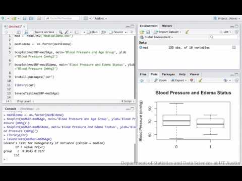
In this example, an ANOVA is performed to determine if mean blood pressure can be explained by age group and presence of edema. Note that this model also tests if the two explanatory variables interact, meaning the effect of one on the response variable varies depending on the level of the other.
Dataset used in video
R script file used in video


Sample conclusion: While controlling for edema status, mean blood pressure does not significantly differ across age groups (F=2.71, df=(2,149), p=0.07). While controlling for age group, mean blood pressure does not significantly differ between patients with and without edema (F=3.05, df=(1,149), p=0.08). Also, there is no interaction between age group and edema status on blood pressure (F=0.68, df=(2,149), p=0.51).
Example 2: Performing a general linear model in R
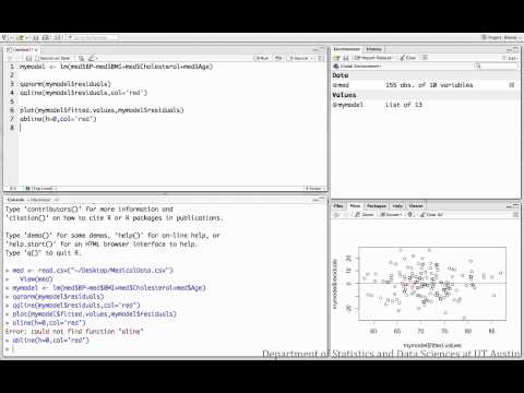
In the following video, a general linear model is run to see if patient’s BMI, cholesterol, and age group significantly explain variation in their blood pressure. Note that similar to Example 1, “age” is a categorical variable, where patients were grouped into being either young adults, adults, or older adults. The regression model chooses an arbitrary reference group (the first alphabetically), and provides estimates for the other two categories, which are the difference in mean blood pressure of each compared to the reference group.
Dataset used in video
R script file used in video


Sample conclusion: While controlling for cholesterol and age group, a patient’s BMI does significantly predict their blood pressure (t=5.88, df=149, p<0.05). While controlling for BMI and age group, cholesterol does not explain blood pressure (t=-.17, df=149, p>0.05). And finally, while controlling for BMI and cholesterol, there is no difference in mean blood pressure between adults and older adults (t=0.53, df=149, p>0.05), but there is a difference in mean blood pressure between adults and younger adults (t=-3.36, df=149, p<0.05).
