A one-way (or single-factor) ANOVA can be run on sample data to determine if the mean of a numeric outcome differs across two or more independent groups. For example, suppose we wanted to know if the mean GPA of college students majoring in biology, chemistry, and physics differ. Note that we could not run a two-sample independent t-test because there are more than two groups.
Hypotheses: (for k independent groups)
Ho: The population means of all groups are equal, or μ1 = μ2 = … = μk
HA: At least one population mean is different, or μi ≠ μj for some i, j
Relevant equations:
Degrees of freedom: Group: k – 1; Error: N – k. Where k is the number of groups and N is the overall sample size.
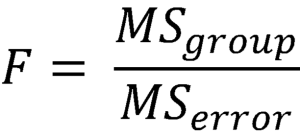
ANOVA, which stands for analysis of variance, separates the overall variance in the outcome into variance explained by the group differences and variance that is within each group (which is the variance unexplained by group). The test statistic, F, is the ratio of the variation in the outcome that is between groups divided by the amount within groups.
The test statistic, F, where MSgroup is the mean squared error of between-group variance and MSerror is the mean squared error of within-group variance:
Assumptions:
- Random samples
- Independent observations
- The population of each group is normally distributed
- The population variances of all groups are equal
If the normality and/or equal variance assumption is violated, the non-parametric Kruskal-Wallis test can be run instead of ANOVA.
Post-hoc testing:
If an ANOVA results in a significant F-statistic, which indicates that there is some difference in means, it’s common to investigate which pairs of groups have significantly different means. Post-hoc testing can accomplish this with pairwise comparison tests (independent t-tests). The number of possible pairwise comparisons is equal to: k(k-1)/2. Due to an increased risk of Type-I errors (rejecting a true null hypothesis), when conducting multiple pairwise tests, it is recommended to use a correction, such as the Bonferroni correction, Fisher’s least significant difference (LSD), or Tukey’s procedure.
Example 1: Hand calculation
This example tests if the mean number of hours worked per week differs across levels of education status.
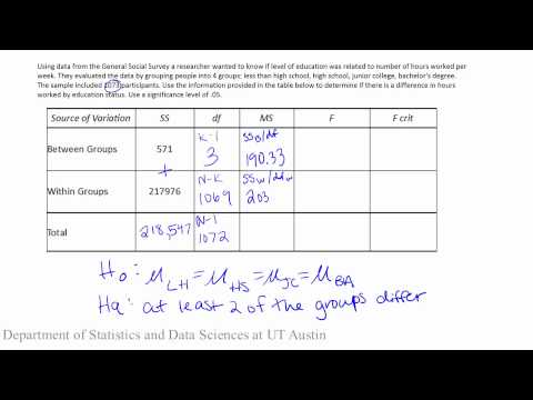

Sample conclusion: There is no indication that the mean number of hours worked per week differs for workers based on their education status (F(df=3,1069)=0.31, p > 0.05).
Example 2: How to run in Excel 2016 on
Some of this analysis requires you to have the add-in Data Analysis ToolPak in Excel enabled.
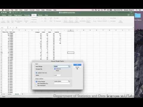
In this video, an ANOVA is run to test if the mean time spent on the phone differs depending on whether students are the oldest, middle, youngest, or only child.
Conducting a one-way ANOVA:
PDF directions corresponding to videos

Conducting post-hoc tests with the Bonferroni correction:
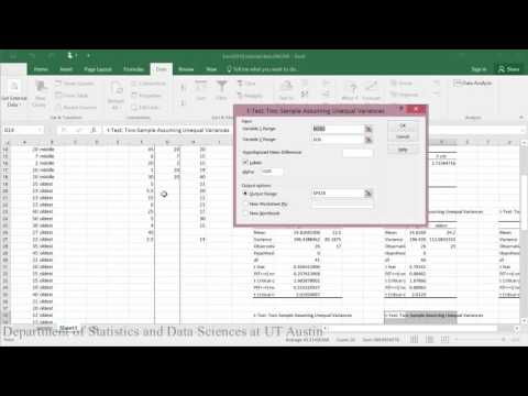

Sample conclusion: With F(df=3,71)=3.63, p<0.05, this data provides evidence that there is a difference in mean phone time based on birth order. After conducting post-hoc testing using a Bonferroni correction, we determined that only the middle and oldest groups significantly differ (p<0.001).
Example 3: How to run in RStudio
This example looks at the mean blood pressure across three different age groups of patients. Notice that age is typically a numeric variable, but in this dataset, each patient’s age was only recorded as belonging to one of three categories: young adult, adult, or older adult.
Dataset used in video
R script file used in video
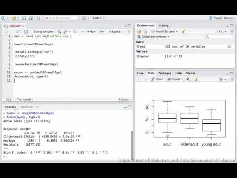

Sample conclusion: With F(df=2,152)=6.40, p<0.05, we find evidence that mean blood pressure is not the same across these three age groups. After conducting post-hoc analysis using a Tukey HSD adjustment, we find that the young adult and adult groups significantly differ (p-value=0.002) and the young adult and older adult groups differ (p-value=0.02)

