Repeated measures ANOVA is used when you have the same measure that participants were rated on at more than two time points. With only two time points a paired t-test will be sufficient, but for more times a repeated measures ANOVA is required. For example, if you wish to track the progress of an exercise program on participants by weighing them at the beginning of the study and then every week after that for 6 weeks (a total of 7 time points) a repeated measures ANOVA would be required. This could also be used if the same participants are put through several conditions, for example, a study may test the effects of different colors of paper on memory. Participants are repeatedly ask to memorize lists of words written on either white, yellow, blue, or pink paper. If each participant goes through each condition, this would also be a repeated measures ANOVA.
One note on the second type of design, for this it is good to counterbalance by ensuring that participants are randomly assigned which color order they go through. Repeated measures tests are subject to issues of practices affects. Which means that participants may get better as they continue to repeat the same test, so randomizing the order of colors ensures order effects are not a confounding factor.
The benefits of repeated measures designs are that they reduce the error variance. This is because for these tests the within group variability is restricted to measuring differences between an individual’s responses between time points, not differences between individuals. Thus, researchers are better able to attribute differences across conditions or time points to being related to treatments or time factors, rather than to individual differences.
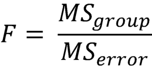
The traditional ANOVA formula is:
The test statistic, F, where MSgroup is the mean squared error of between-group variance and MSerror is the mean squared error of within-group variance. When the repeated measures ANOVA is calculated the MSgroup is split in to two parts: the between-subjects variability and what variations remains after that. The final calculation subtracts the between-subjects variability which typically reduces the MSerror significantly, thus giving the test more power.
Assumptions:
- Random samples
- Independent observations
- Multivariate normality – there are normally distributed population values for each measure
- Sphericity – all differences between pairs of scores are equally variable (see video for details)
Example: Performing a repeated measures ANOVA in R
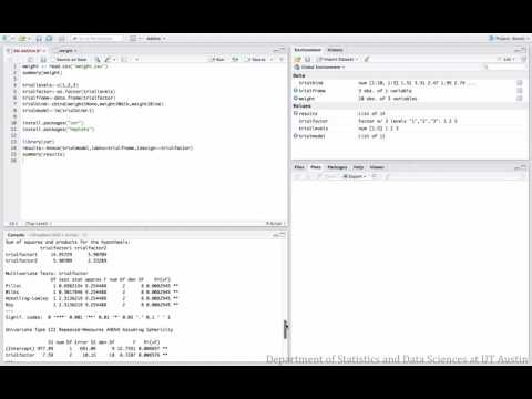
In the following video, a repeated measures ANOVA is run to see if participants’ weight loss differs between a weight loss therapy program only, the program plus a walking regimen, or the program plus a biking regimen.
Dataset used in video
R script file used in video


Sample conclusion: After completing the repeated measures ANOVA we did find that there were differences for participants’ weight loss depending on the type of weight loss program they underwent (F(2,18)=6.73, p=.02). Using post-hoc testing with a Bonferroni correction we found that participants’ weight loss was significantly less with the no additional treatment than with the additional biking regimen (p=.04), or the walking regimen (p=.009), but the walking and biking regimen weight loss did not significantly differ (p=.74).

