
The SPACE program: Stochastic Population Analysis for Complex Events (May 15, 2018)
Introduction
The SPACE (Stochastic Population Analysis for Complex Events) program is a package of SAS programs to compute health expectancy (HE) via a multi-state life table (MSLT). The MSLT model follows a first-order Markov process where the transition probabilities depend on the current status only. The SPACE program also allows for the computation of standard errors for the estimated HE using the bootstrap method (Rao and Wu 1988), which has been used in two previous studies (Cai and Lubitz 2007; Cai et al. 2006) and is described in detail in a manuscript (Cai et al. 2010).
The SPACE program offers users various options to calculate HE. The estimation can be performed with or without the covariates, which are not limited to be dichotomous. It allows users to choose the appropriate method to estimate the transition probabilities and rates (multinomial logistic regression or hazard regression). It also provides different ways to calculate HE – the deterministic approach or the stochastic approach (i.e., microsimulation). Simulation offers users a high degree of flexibility to summarize various aspects of the dynamics of population health changes.
The SPACE program has two main sets of programs, offering users different possible combinations of the available functions. The two sets estimate a first-order Markov model:
- Module 1 (RAD files) estimates age-specific state-dependent transition rates using the discrete-time hazard model and calculates HE using the deterministic approach
- Module 2 (SIM files) estimates age-specific state-dependent transition probabilities (or rates) using the multinomial logistic regression (or the discrete-time hazard model) and calculates MSLT functions (including HE) using microsimulation.
Each set of programs has two components: xxx_M and xxx_S. The xxx_M program is the main control program, while the xxx_S is the main statistical program. The xxx_M program first launches the xxx_S program to calculate the point estimates from the full analysis data sample (indexed by BS=0). It then generates a large number of bootstrap samples and calculates the life table (LT) functions for each of the samples (indexed by BS>=1). The standard errors of the original point estimates are the standard deviations of these bootstrap estimates.
Users with multi-CPU computers can use Module 2 which has the ability to provide an estimation of MSLT function for the bootstrap samples in batches. The current version executes multiple sessions of SAS simultaneously for computers equipped with multiple CPUs. Note that in order to execute multiple sessions of SAS simultaneously, the users must have SAS/Connect installed on their computer. In my experience, it is necessary to avoid using all CPU cores, and it is better to leave at least two CPU cores for the Windows system to use.
In what follows, I will describe in more detail how these programs work, and the type of data sets these programs require.
Before running the program
- The SPACE program requires SAS/IML (Interactive Matrix Language). If you do not have IML installed on your computer, please install it first.
- The SPACE program is developed and tested in PC SAS 9.1.3, 9.2, 9.3 and 9.4. It has not been tested in earlier versions. The most up-to-date version is coded in SAS 9.4 in 64-bit Windows. Note: 32 bit and 64 bit SAS data files seem to have some compatibility issues.
- In order to run the program, please put all SPACE program files and your SAS data file in the same folder. However, due to a known issue, please do NOT put SPACE program in a long-long-name folder under many-many-level parent folders because doing so will cause unknown errors in SAS.
Data
The data set should be prepared like the example data set. Each interview observation should occupy one line of record in the data set. The xxx_S program will convert these records into the format of annual (not 12-month) intervals for transition probability or transition rate estimation. The interviews need not be equally spaced; the length of time between interviews can vary, as long as it is longer than one year.[1] If the survey has interview gaps of two or more years, then pseudo interview data will be created to “fill in” the unobserved years. If the states occupied in the two successive interviews are different, then an event is assumed to have occurred randomly between the two interviews. For example, if the interviews were conducted in 2000 and 2004, then the timing of the event would be randomly assigned to 2001, 2002 or 2003 with the probability of 1/3. If the observed states are identical at two successive interviews, then no event is assumed to have occurred. Below is a simple example focusing on age and health outcomes.
Supposed that we have a wide-form panel data:
| ID | Age1 | Age2 | Age3 | D_age | Sex | S1 | S2 | S3 | (other variables) |
| 1 | 60 | 62 | 64 | . | 1 | 2 | 2 | 2 | |
| 2 | 52 | 54 | 56 | . | 2 | 2 | 2 | 1 | |
| 3 | 78 | 80 | 82 | . | 1 | 1 | 1 | 2 | |
| 4 | 50 | 52 | . | 53 | 1 | 2 | 1 | . | |
| 5 | 83 | . | . | 84 | 2 | 2 | . | . |
Next, we need to convert the data from wide form to the long form as below to run incidence-base multistate life tables.
| ID | Age | Sex | S | HSQ | (other variables) |
| 1 | 60 | 1 | 2 | 2 | |
| 1 | 62 | 1 | 2 | 2 | |
| 1 | 64 | 1 | 2 | 2 | |
| 2 | 52 | 2 | 2 | 2 | |
| 2 | 54 | 2 | 2 | 2 | |
| 2 | 56 | 2 | 1 | 1 | |
| 3 | 78 | 1 | 1 | 1 | |
| 3 | 80 | 1 | 1 | 1 | |
| 3 | 82 | 1 | 2 | 2 | |
| 4 | 50 | 1 | 2 | 2 | |
| 4 | 52 | 1 | 1 | 1 | |
| 4 | 53 | 1 | . | 3 | |
| 5 | 83 | 2 | 2 | 2 | |
| 5 | 84 | 2 | . | 3 |
Then, HSQ (1=healthy, 2=unhealthy, 3=dead) will be the health outcome variable in SPACE. The input data has to have no missing of all necessary variables during estimation. For example, ID, Age, Sex, HSQ, Sample_weight, PSU, Strata. In the above example, SPACE will not use S during estimation; it is fine to have some missing values for S or you can just delete it. Please note that:
- ID has to be “ID” in the input data, but lower or upper case doesn’t matter.
- Age has to be “Age” in the input data, but lower or upper case doesn’t matter.
- If you don’t have Strata and PSU (primary sampling unit) variable in your own data, you can create the two variables by assigning Strata=1 and PSU=ID in the data.
- The name of health variable can NOT be “HS” or “ID” or “Age”.
- The values of covariates (e.g., Sex) in the input data have to start from 1 (NOT 0) and then 2, 3, 4,…etc.. It has also to be consecutive numbers starting from 1. For example, if the variable has 3 categories, its values have to be 1,2,3, and it can’t be like 1,3,4.
- Even covariates are dummies (with values of 0 or 1), that is to say, the values have to be changed so that the values start from 1. You can see the values of “Sex” in the above example.
- The number of health states in your data can exceed 3 in the simulation program. But death should always be indicated by the largest integer in the defined state space. The values of health variable have to start from 1.
[1] If the survey has more frequent interviews, the SPACE program will need to be modified. Please contact Chi-Tsun Chiu for such problems.
Define macro variables in SPACE_macro.sas
In the SPACE_macro.sas file, users have to define macro variables before running SPACE.
(1)All programs
- BSIZE: the number of bootstrap samples. The value is 0 or any positive integer bigger than 1, where 0 means no bootstrap sample, and only point estimates will be presented in output files. If inputting 1, SPACE will change it back to 0.
- BEG: the first age interval of the life table. This has to be an integer, and this is age in year.
- AgeLowerLimit: the lowest age from the input data.
- Datainput: the name of SAS input data
- depVAR: the dependent variable (Health state variable). Can NOT use “HS”.
- STRATCOV: the list of covariate(s) used to stratify the analysis. Separate each with a blank space. A blank space means no stratification variable.
- REGCOV: the list of covariate(s) in regression models. Separate each with a blank space. A blank space means no covariate except Age variable in the model.
- TVcov: the list of time-varying covariate(s). Must be categorical, and part of REGCOV.
- STRATA: STRATA variable.
- PSU: PSU variable.
- WGT: sample weight.
- TXT_output: 1 (default): Generate the tab separated TXT output files that EXCEL can open. 0: NO. However, output files of SAS format data will always be generated.
Note: if TXT_output=1, you may have to use -noterminal option under Unix-like platform.
- nHealthState: the number of health states (including the absorbing state). Default is 3 (e.g., 2 living health states + 1 dead state). Only SIM (2+) can you change this. Note: when nHealthState=2, it’s a traditional life table.
- Subset: the dichotomized variable (0/1) for subset of the input data set. SPACE will only use data with Subset value=1. Default is blank (ie., whole data).
- randomSeed: random number seed: 1 = DateTime(); 0 = BS, ie., the index of each bootstrap sample (seed=1 for 1st bootstrap sample, seed=2 for 2nd bootstrap sample, etc.). Default is 0. Using 0 allows you to replicate results each time you run SPACE with identical settings.
- InteractionTerm: user-defined interaction terms. Default is blank. For example,
- If users would like to include an interaction term between Age and Sex
- Age*Sex
- If users would like to include an interaction term between Age and Sex, and an interaction term between Sex and Education
- Age*Sex Sex*Education
- If users would like to include an interaction term between Age and Sex
- AGE_sq: 1 = having an age squared term; 0, otherwise. Default = 0.
(2)RAD programs (Module 1) only
- END_LT: the last age (open interval) of the life table.
(3)SIM program (Module 2) only
- SIMSIZE: size of simulation cohort.
- d_BEG: range of age in the output. If only need AGE=BEG in the output, put 0 here.
- d_AGE: the increment of first age across life tables. Can NOT be 0. At least 1.
- For example,
- If users would like to have HE outputs at 65 only, the settings are
- BEG = 65, d_BEG=0. Note: d_AGE doesn’t matter.
- If users would like to have HE outputs at 65, 75, 85, the settings are
- BEG = 65, d_BEG=20 (=85-65), d_AGE=10 (=75-65=85-75).
- If users would like to have HE outputs at 65 only, the settings are
- logitHazard: 1=Logit model (Default), 2=Hazard model.
- nSession: the number of sessions (2+) for parallel computation under a multi-CPU computer. Without SAS/CONNECT, it has to be 1.
Note: please make sure your computer has SAS/CONNECT installed.
- NoTrans: specify transitions that are not allowed. Default is blank. For example,
- B3E1 B3E2
- B: beginning state; E: ending state
- B3E1: transition from state 3 to state 1
- Transitions separated by blank spaces
- Has to be numeric and less than nHealthState – 1
- B3E1 B3E2
- SimLifeLine: whether to save simulation outputs: 0=No (Default). 1=Yes.
- CtrlCOVmodel: Whether use control variable(s) in regression models: 0=No (Default). 1=Yes.
- CtrlCOVcateg: Categorical control variable(s) in the regression model.
- CtrlCOVconti: Continuous control variable(s) in the regression model.
- Note:
- The values of control variables do not need to start from 1. You can input in the common way that SAS Proc Logistic can accept in the regression model.
- To include control variables in analyses, you need to assign CtrlCOVmodel=1 and put at least one variable’s name in either CtrlCOVcateg or CtrlCOVconti.
Note:
- The covariates listed in STRATCOV or REGCOV have to be categorical variables with values starting from 1 (Not 0).
- Please remove all format in SAS data file to prevent unexpected errors. The SAS code is:
proc datasets lib=YourLibrary;
modify InputDataName;
format _all_;
informat _all_;
run;
For example, C:\SPACE\sample.sas7bdat
%Let S = C:\SPACE; → S is the library name;
“sample” is the input data name;
- If users encounter the compatibility issues between 32 bit and 64 bit SAS data files, please use software like StatTransfer to transfer SAS data file to other data format (eg., Stata (.dta), ASCII/Text-Delimited (.csv)) and transfer back to SAS data format. Or users can try any other way that can remove all format or 32bit/64bit related issue from the input data.
Output files
There are several SAS and TXT output data files generated by SPACE.
For example, if BEG=65, END_LT=100, BSIZE=250, SIMSIZE=100000, nHealthState=3, depVAR=HSQ,
(1)Health Expectancy (TXT files) (if TXT_output=1 in the SPACE_macro.sas)
- SPACEmodule = 1
- RAD_A65_100b250.txt: TLE, ALE, DLE with standard errors at age 65-100
- State=0: population-based estimation
- State=1 or 2: status-based estimation (from depVAR value = 1 or 2)
- TLE: total life expectancy (from depVAR value = 3)
- ALE: active life expectancy (from depVAR value = 1)
- DLE: disable life expectancy (from depVAR value = 2)
- TLE_STD: standard error for TLE
- ALE_STD: standard error for ALE
- DLE_STD: standard error for DLE
- RAD_A65b250.txt: TLE, ALE, DLE with standard errors at age 65
- (Same as RAD_A65_100b250.txt)
- RAD_A65_100b250.txt: TLE, ALE, DLE with standard errors at age 65-100
- SPACEmodule = 2
SIM_A65s100000b250.txt
- Age: the first age of the life table
- State=0: population-based estimation
- State=1,2,3,…: status-based estimation (from depVAR value = 1,2,3,…)
- TLE: total life expectancy (from depVAR value = nHealthState)
- LEs1: life expectancy with depVAR value = 1
- LEs2: life expectancy with depVAR value = 2
- ….etc.
- XXX_STD: the standard error of XXX. For example,
- TLE_STD: the standard error of TLE
(2)Health Expectancy (SAS data files)
- SPACEmodule = 1
RAD_LE.sas7bdat: results from all bootstrap samples
- BS=0: point estimates from the full analysis data sample
- BS>=1: point estimates from each bootstrap sample
-
RAD_LESTD.sas7bdat: is RAD_A65_100b250.txt
-
RAD_LESTD_A65.sas7bdat: is RAD_A65b250.txt
- SPACEmodule = 2
SIM_LE.sas7bdat: results from all bootstrap samples
- BS=0: point estimates from the full analysis data sample
- BS>=1: point estimates from each bootstrap sample
- SIM_LESTD.sas7bdat: is SIM_A65s100000b250.txt
(3)Coefficients (lst files)
- SPACEmodule = 1
-
RAD_Lifereg_HSQ_B1E2.lst
-
RAD_Lifereg_HSQ_B1E3.lst
-
RAD_Lifereg_HSQ_B2E1.lst
-
RAD_Lifereg_HSQ_B2E3.lst
- Note: BiEj indicates the transition from i to j
-
- SPACEmodule = 2
- if logitHazard=1 (transition probability)
-
SIM_Logistic_trans_HSQ.lst
-
- if logitHazard=2 (transition rate)
- SIM_Lifereg_HSQ_B1E2.lst
- SIM_Lifereg_HSQ_B1E3.lst
- SIM_Lifereg_HSQ_B2E1.lst
- SIM_Lifereg_HSQ_B2E3.lst
- Note: BiEj indicates the transition from i to j
- if logitHazard=1 (transition probability)
(4)Simulated life lines (if SimLifeLine=1 in the SPACE_macro.sas)
- SPACEmodule = 2
- Sim_LifeLines.sas7bdat: all detailed simulated life lines
- Sim_SumLifeLines.sas7bdat: all summary simulated life lines
(5)Log files
- SPACEmodule = 1, 2
-
SPACE.log: include all the detail SAS log that is useful for debug.
- Normally its size does not exceed 100MB, and it is often less than 10MB for a simple model. If the size is strangely large with only a small run, there is something seriously wrong. Please check the log file first (if you can still open it) to see where the problem it. However, if you can’t even open it due to the large size of log file, please check SPACE_macro file and the input data.
-
- SPACEmodule = 2 (if nSession >1 in the SPACE_macro.sas)
-
BSMSlog1.LOG: the log file from parallel remote session
-
BSMSlog2.LOG: the log file from parallel remote session
-
…etc.
- Note:
- The total number of remote sessions and their log files is the value of nSession in the SPACE_macro.sas
- SAS/Connect is required to perform parallel computation
-
Run SPACE
(1)Put all SPACE program files and your input data all together in one folder, say, C:\SPACE.
(2)Open SPACE_macro.sas.
- Modify all parameters that you need for the analysis.
(3)Open SPACE_MAIN.sas
- Modify the path where you put all SPACE program files and the input data. For example,
- %let workpath = C:\SPACE ; (please do not use ” or ‘.)
- Note: please do NOT put SPACE program in a long-long-name folder under many-many-level parent folders because doing so will cause unknown errors in SAS.
- Change the module value: 1 for deterministic approach; 2 for simulation approach.
(4)Click the small running person icon on the top of SAS to run SPACE under the page of SPACE_MAIN.sas.
Open TXT output files with EXCEL for the first time
To open the output TXT file with EXCEL for the first time, you need to tell Windows that Excel can open it.
Please go to the file, mouse right-click the TXT file → Open with → Choose default program.
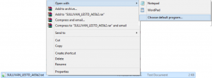
Below will be what you see. Uncheck “Use this app for all .txt files” and click “More options”.

If you cannot see Excel on the list, click “Look for another app on this PC”.

Please go to “C:/Program Files/Microsoft Office/Office16” (folder name is dependent on what version of MS Office you have in your PC), click EXCEL.EXE and then “Open”.
Note: the folder may be slightly different due to different versions of Microsoft Office, and it could be under “C:\Program Files (x86)\…”

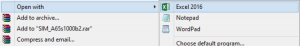
Mouse right-click the TXT file→ Open with. If you can see EXCEL, you can now use EXCEL to open it (as below).
Note1: Please do remember to close the TXT file opened by EXCEL before running SPACE. It is better to close EXCEL before running SPACE if EXCEL has been opening any SPACE TXT output file; failure to do so means EXCEL will lock the file and SPACE will not have the right to make any changes to the file.
Note2: If you put SPACE program in a Dropbox folder, please remember to pause Dropbox before running SPACE; otherwise Dropbox will lock some SAS data files and SAS will be unable to revise those files.
The example data set
In the “sample.sas7bdat” data set, these variables are included (some variables are mandatory for any input data set. They are marked by *.):
- ID*: personal identifier.
- Age*: age at interview (or death).
- Sex: 1=male, 2=female.
- W1married: 1=not married at w1, 2=married at w1.
- Hi_schl_up: 1=below high school, 2=high school and above.
- Urban12: 1=not live in urban, 2= living in urban.
- HST*: categorical and mutually exclusive health measure (1=active, 2=disabled with 1+ IADL or ADL limitations, 3=dead). Please note that the number of health states in your study can exceed 3. Death should always be indicated by the largest integer in the defined state space.
- Strata*: indicator of strata in the sample. Here Strata is 1.
- PSU*: indicator of PSUs in the sample. Here PSU is ID.
- Wgt*: sample weight for the current observation.
- Wave: interview waves.
Please note that the bootstrap samples are generated only from the first-stage sampling (i.e., at the PSU level). If the original survey is a stratified simple random sample, then the PSU variable should be identical to the ID variable so that individuals are treated at PSUs and are selected.
Program overview
MSLT_RADxCOV_M and MSLT_RADxCOV_S
The MSLT_RADxCOV_M launches the MSLT_RADxCOV_S program to estimates HE from the full analysis sample and bootstrap samples. The RADxCOV programs estimates MSLT functions conditional on age only or one or more covariates.
Please note that the bootstrap samples are generated at PSU level. Once a PSU is selected, all sampled persons in that PSU are included in the bootstrap sample and their weights are recalculated by the number of time their PSUs are selected. Also, if there is only a single PSU in a particular stratum, then this single PSU is selected with certainty.
MSLT_SIMxCOV_M and MSLT_SIMxCOV_S
The MSLT_SIMxCOV_M launches the MSLT_SIMxCOV_S program to estimates HE from the full analysis sample and bootstrap samples. The SIMxCOV programs estimates MSLT functions conditional on age only or one or more covariates. It has three major differences from the RADxCOV program.
(1) The SIMxCOV estimates either transition probabilities using a multinomial logistic regression (Allison 1982; Allison 1984) or transition rates using a hazard model, while the RADxCOV program only estimates a transition rates using a hazard model.
(2) The SIMxCOV program estimate a variety of MSLT functions via simulation, while the RADxCOV program estimates HE only using the deterministic approach. Simulation produces a large collection of individual health trajectories, and offers researchers much greater flexibility to summarize the dynamics of population health.
(3) The SIMxCOV program simulates a single large cohort for each age. Each cohort is distributed by the health status and covariates measured at the baseline of survey. The RADxCOV program estimate HE separately for each combination of the levels of the covariates.
Summary
This manual only provides a brief overview of the SPACE program. It is strongly recommended that users test the programs on their computer first using the example data to become familiar with the program. I will provide as much as trouble shooting as my time allows, but I cannot guarantee to respond to your questions within a certain time window. Please email your questions to me at ctchiu at gate.sinica.edu.tw.
Enjoy!
Best,
——————————————————–
Note: This manual is directly revised from Dr. Liming Cai’s original SPACE manual (June 23, 2009) and reflects my modifications in the SPACE program.
——————————————————–
Get the PDF copy of complete SPACE_manual.
Get all SPACE program files here.
Note: A new version of the SPACE program in R/C++ is available here.
Note: If you can’t access Dropbox you can contact me directly by email (ctchiu at gate.sinica.edu.tw) for a copy of the SPACE program.
Reference:
- Allison, P.D. 1982. “Discrete-Time Methods for the Analysis of Event Histories.” Pp. 61-98 in Sociological Methodology.
- Allison, P.D. 1984. Event history analysis : regression for longitudinal event data. Beverly Hills, Calif.: Sage Publications.
- Cai, L., M. Hayward, Y. Saito, J. Lubitz, A. Hagedorn, and E. Crimmins. 2010. “Estimation of multi-state life table functions and their variability from complex survey data using the SPACE Program.” Demographic Research 22(6):129-158.
- Cai, L.and J. Lubitz. 2007. “Was There Compression of Disability for Older Americans From 1992 to 2003?” Demography 44(3):479-495.
- Cai, L., N. Schenker, and J. Lubitz. 2006. “Analysis of functional status transitions by using a semi-Markov process model in the presence of left-censored spells.” Journal of the Royal Statistical Society: Series C (Applied Statistics) 55(4):477-491.
- Rao, J.N.K.and C.F.J. Wu. 1988. “Resampling Inference with Complex Survey Data.” Journal of the American Statistical Association 83(401):231-241..