
A two-sample independent t-test can be run on sample data from a normally distributed numerical outcome variable to determine if its mean differs across two independent groups. For example, we could see if the mean GPA differs between freshman and senior college students by collecting a sample of each group of students and recording their GPAs.
Hypotheses:
Ho: The population mean of one group equals the population mean of the other group, or μ1 = μ2
HA: The population mean of one group does not equal the population mean of the other group, or μ1 ≠ μ2
This test can also be conducted with a directional alternate hypothesis:
Ho: The population mean of one group equals the population mean of the other group, or μ1 = μ2
Ha: The population mean of one group is greater than the population mean of the other group, or μ1 > μ2
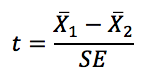
The test statistic for a two-sample independent t-test is calculated by taking the difference in the two sample means and dividing by either the pooled or unpooled estimated standard error. The estimated standard error is an aggregate measure of the amount of variation in both groups.
Relevant Equations:
Degrees of freedom: Varies by conditions, but the basic rule of thumb for hand calculations is the smaller of n1 – 1 and n2 – 1, where n is the sample size for each group.
Assumptions:
- Random samples
- Independent observations
- The population of each group is normally distributed.
- The population variances are equal.
If the third assumption is not met, the alternative test is the Mann-Whitney U-Test, which can be run to see if there is a difference between two groups for a variable with any type of distribution.
If the fourth assumption is met, then the pooled estimated standard error is used in the calculation of the test statistic. If the fourth assumption fails, then the more conservative unpooled estimated standard error is used (and the test is referred to as “Welch’s Test”).
Example 1: Hand calculation video
This example looks at the mean number of hours slept for male versus female students.
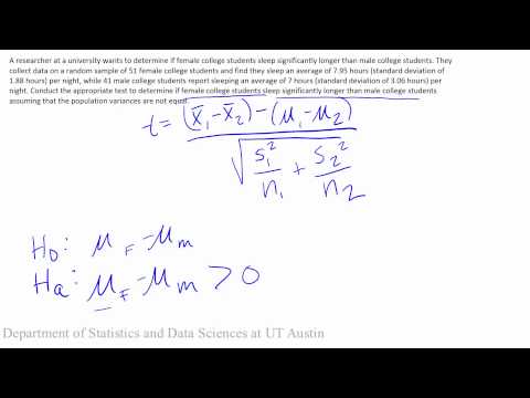

Sample conclusion: With t(df=40)=1.73, which was more extreme than our critical value of 1.68, this data does provide evidence that female students do sleep more, on average, than male students.
Example 2: How to run in Excel 2016 on
Some of this analysis requires you to have the add-in Data Analysis ToolPak in Excel enabled.
In this tutorial, you will determine if males and females differ in their level of happiness.
NOTE: In this video, the t-test is conducted assuming unequal variances (Welch’s Test).
Dataset used in video
PDF directions corresponding to video
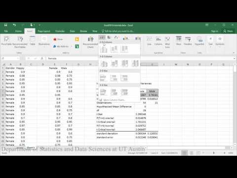
Sample conclusion: With t(df=28)=2.29, p<0.05, this data does provide evidence that female students are happier, on average, than male students.
Example 3: How to run in RStudio
This example looks at the mean number of hours slept for male versus female students.
NOTE: In this video, the t-test is conducted assuming unequal variances (Welch’s Test).
Dataset used in video
R script file used in video
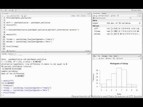
Sample conclusion: With t(df=27)=-0.42, p>0.05, we found no evidence to suggest that male and female students sleep different amounts, on average, on Tuesday nights.