This was a keynote presentation at the “2nd International Workshop on Performance Modeling: Methods and Applications” (PMMA16), June 23, 2016, Frankfurt, Germany (in conjunction with ISC16).
The presentation discusses a family of simple performance models that I developed over the last 20 years — originally in support of processor and system design at SGI (1996-1999), IBM (1999-2005), and AMD (2006-2008), but more recently in support of system procurements at The Texas Advanced Computing Center (TACC) (2009-present).
More notes interspersed below….
Most of TACC’s supercomputer systems are national resources, open to (unclassified) scientific research in all areas. We have over 5,000 direct users (logging into the systems and running jobs) and tens of thousands of indirect users (who access TACC resources via web portals). With a staff of slightly over 175 full-time employees (less than 1/2 in consulting roles), we must therefore focus on highly-leveraged performance analysis projects, rather than labor-intensive ones.
An earlier presentation on this topic (including extensions of the method to incorporate cost modeling) is from 2007: “System Performance Balance, System Cost Balance, Application Balance, & the SPEC CPU2000/CPU2006 Benchmarks” (invited presentation at the SPEC Benchmarking Joint US/Europe Colloquium, June 22, 2007, Dresden, Germany.
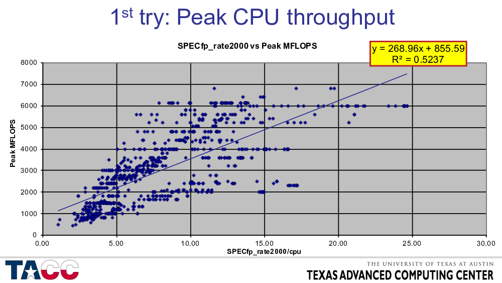
This data is from the 2007 presentation. All of the SPECfp_rate2000 results were downloaded from www.spec.org, the results were sorted by processor type, and “peak floating-point operations per cycle” was manually added for each processor type. This includes all architectures, all compilers, all operating systems, and all system configurations. It is not surprising that there is a lot of scatter, but the factor of four range in Peak MFLOPS at fixed SPECfp_rate2000/core and the factor of four range in SPECfp_rate2000/core at fixed Peak MFLOPS was higher than I expected….
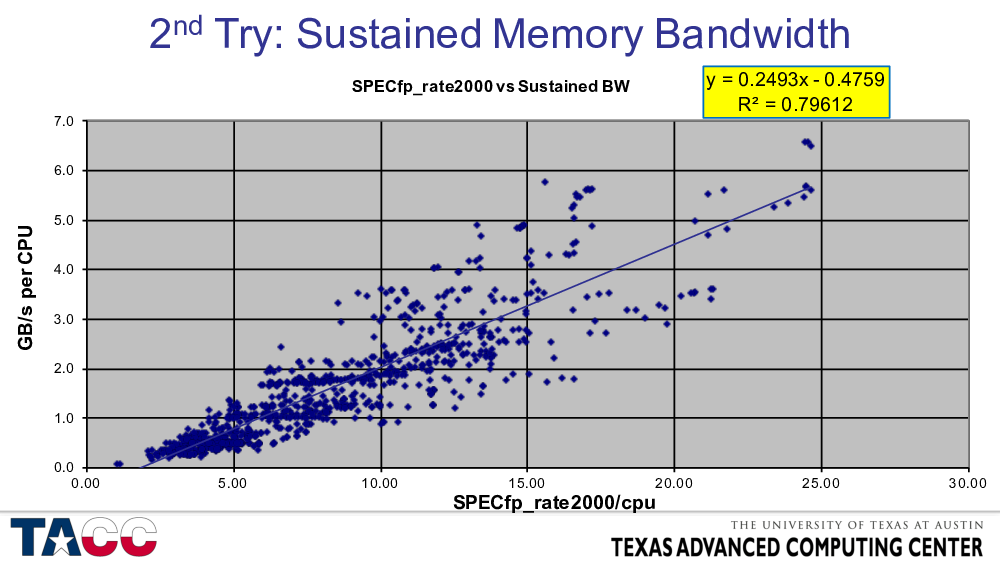
(Also from the 2007 presentation.) To show that I can criticize my own work as well, here I show that sustained memory bandwidth (using an approximation to the STREAM Benchmark) is also inadequate as a single figure of metric. (It is better than peak MFLOPS, but still has roughly a factor of three range when projecting in either direction.)
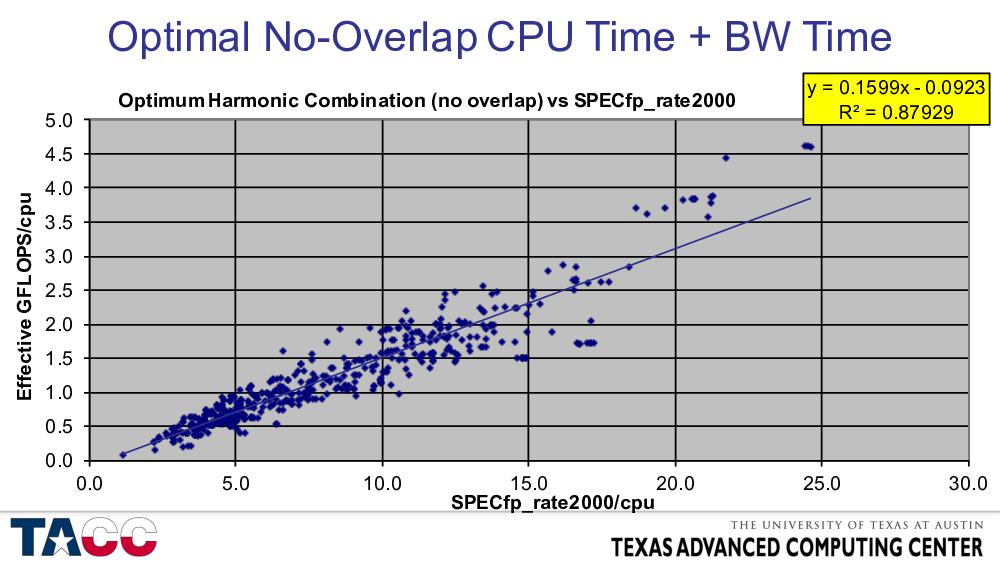
Here I assumed a particular analytical function for the amount of memory traffic as a function of cache size to scale the bandwidth time.
Details are not particularly important since I am trying to model something that is a geometric mean of 14 individual values and the results are across many architectures and compilers.
Doing separate models for the 14 benchmarks does not reduce the variance much further – there is about 15% that remains unexplainable in such a broad dataset.
The model can provide much better fit to the data if the HW and SW are restricted, as we will see in the next section…

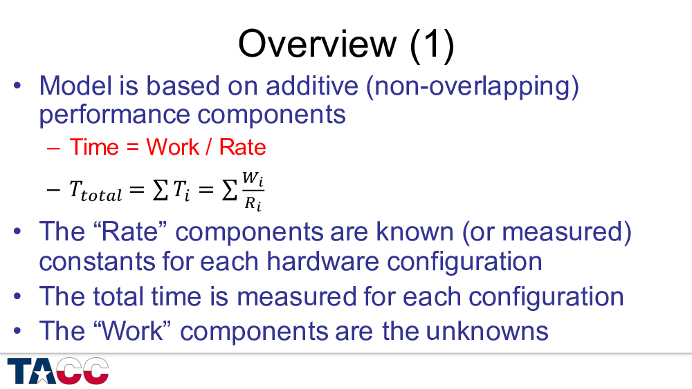
Why no overlap? The model actually includes some kinds of overlap — this will be discussed in the context of specific models below — an can be extended to include overlap between components. The specific models and results that will be presented here fit the data better when it is assumed that there is no overlap between components. Bounds on overlap are discussed near the end of the presentation, in the slides titled “Analysis”.
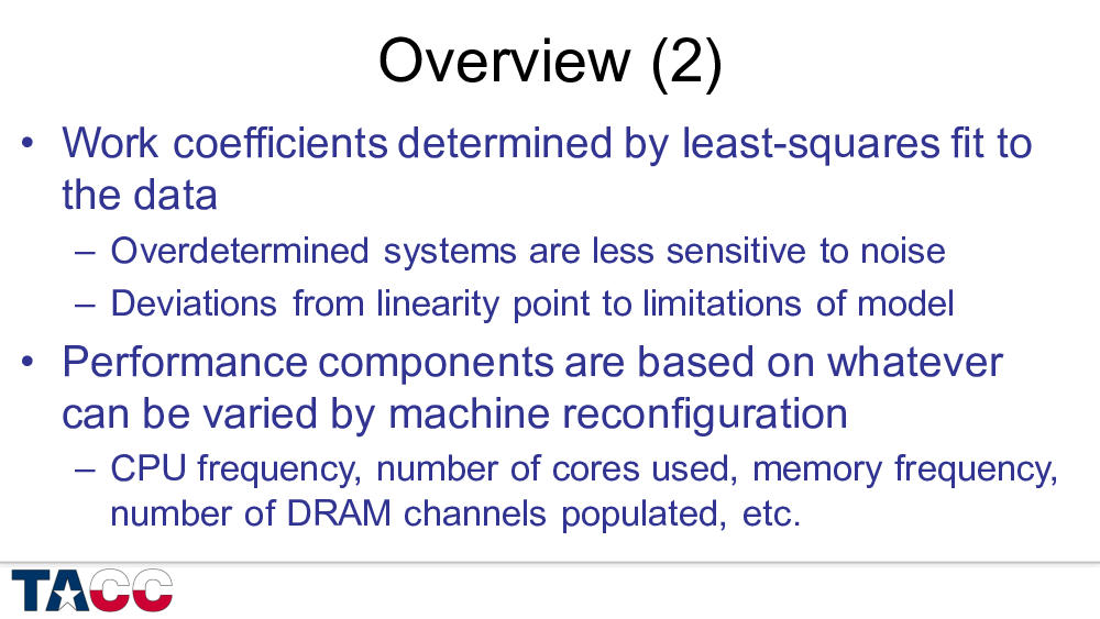
The approach is opportunistic. When I started this work over 20 years ago, most of the parameters I was varying could only be changed in the vendor’s laboratory. Over time, the mechanisms introduced for reducing energy consumption (first in laptops) became available more broadly. In most current machines, memory frequency can be configured by the user at boot time, while CPU frequency can be varied on a live system.
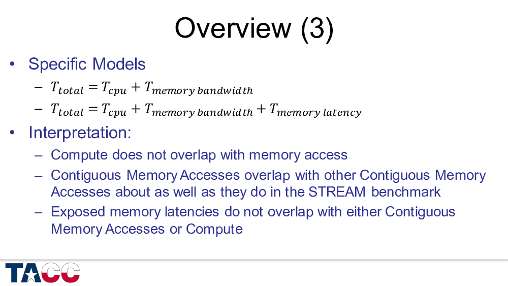
The assumption that “memory accesses overlap with other memory accesses about as well as they do in the STREAM Benchmark” is based on trying lots of other formulations and getting poor consistency with observations.
Note that “compute” is not a simple metric like “instructions” or “floating-point operations”. T_cpu is best understood as the time that the core requires to execute the particular workload of interest in the absence of memory references.

Only talking about CPU2006 results today – the CPU2000 results look similar (see the 2007 presentation linked above), but the CPU2000 benchmark codes are less closely related to real applications.
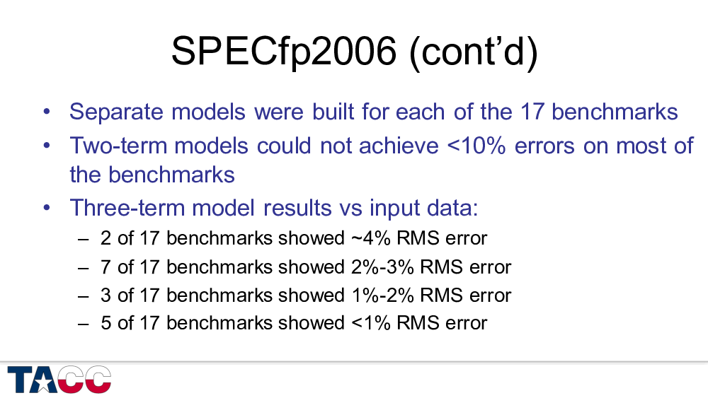
Building separate models for each of the benchmarks was required to get the correct asymptotic properties. The geometric mean used to combine the individual benchmark results into a single metric is the right way to combine relative performance improvements with equal weighting for each code, but it is inconsistent with the underlying “physics” of computer performance for each of the individual benchmark results.
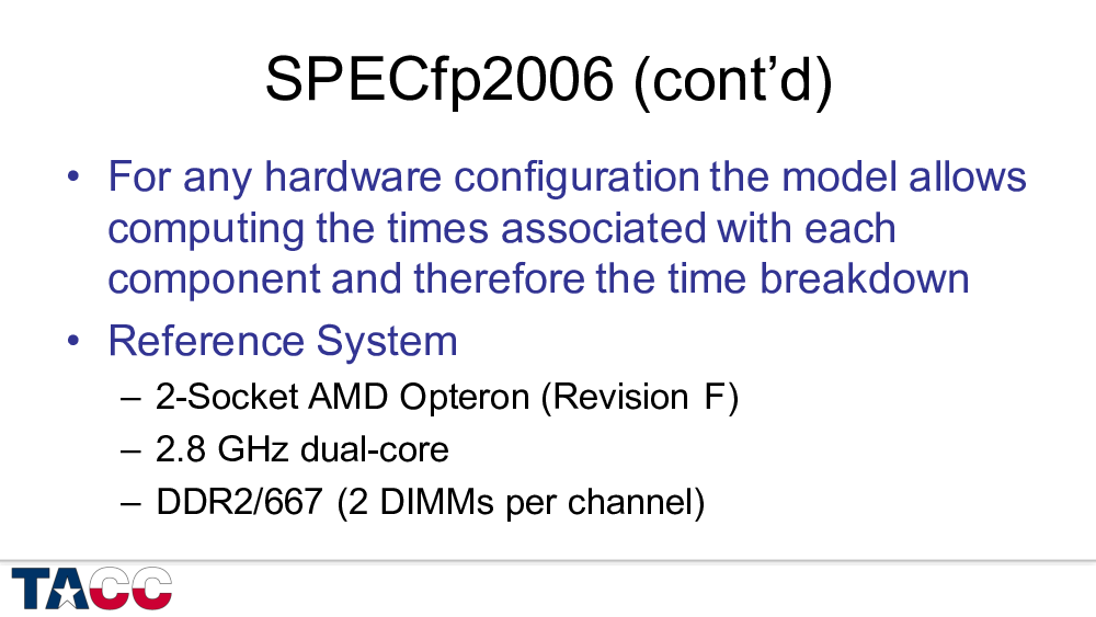
This system would be considered a “high-memory-bandwidth” system at the time these results were collected. In other words, this system would be expected to be CPU-limited more often than other systems (when running the same workload), because it would be memory-bandwidth limited less often. This system also had significantly lower memory latency than many contemporary systems (which were still using front-side bus architectures and separate “NorthBridge” chips).
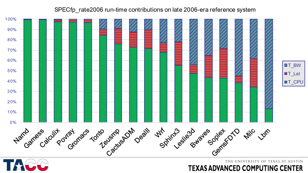
Many of these applications (e.g., NAMD, Gamess, Gromacs, DealII, WRF, and MILC) are major consumers of cycles on TACC supercomputers (albeit newer versions and different datasets).
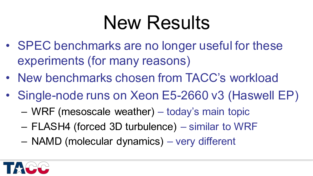
The published SPEC benchmarks are no longer useful to support this sensitivity-based modeling approach for two main reasons:
- Running N independent copies of a benchmark simultaneously on N cores has a lot of similarities with running a parallelized implementation of the benchmark when N is small (2 or 4, or maybe a little higher), but the performance characteristics diverge as N gets larger (certainly dubious by the time on reaches even half the core count of today’s high-end processors).
- For marketing reasons, the published results since 2007 have been limited almost exclusively to the configurations that give the very best results. This includes always running with HyperThreading enabled (and running one copy of the executable on each “logical processor”), always running with automatic parallelization enabled (making it very difficult to compare “speed” and “rate” results, since it is not clear how many cores are used in the “speed” tests), always running with the optimum memory configuration, etc.
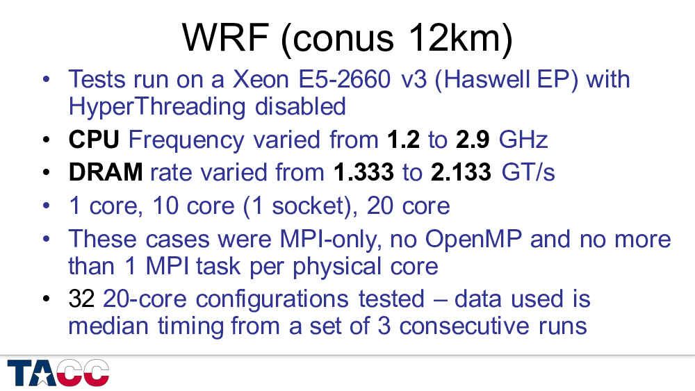
The “CONUS 12km” benchmark is a simulation of the weather over the “CONtinental US” at 12km horizontal resolution. Although it is a relatively small benchmark, the performance characteristics have been verified to be quite similar to the “on-node” performance characteristics of higher-resolution test cases (e.g., “CONUS 2.5km”) — especially when the higher-resolution cases are parallelized across multiple nodes.
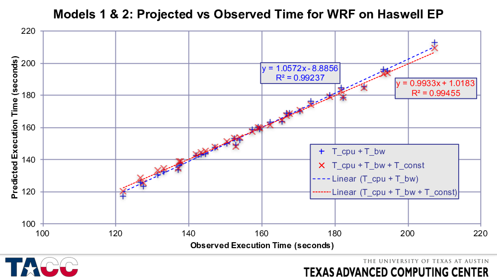
Note that the execution time varies from about 120 seconds to 210 seconds — this range is large compared to the deviations between the model and the observed execution time.
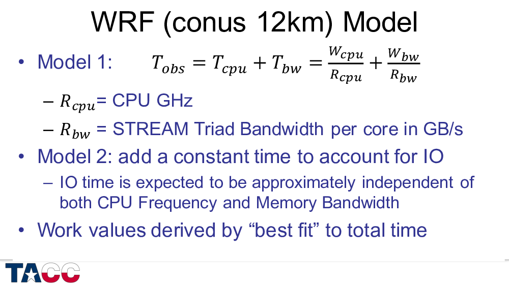
Note also that the slope of the Model 1 fit is almost 6% off of the desired value of 1.0, while the second model is within 1%.
- In the 2007 SPECfp_rate tests, a similar phenomenon was seen, and required the addition of a third component to the model: memory latency.
- In these tests, we did not have the same ability to vary memory latency that I had with the 2007 Opteron systems. In these “real-application” tests, IO is not negligible (while it is required to be <1% of execution time for the SPEC benchmarks), and allowing for a small invariant IO time gave much better results.
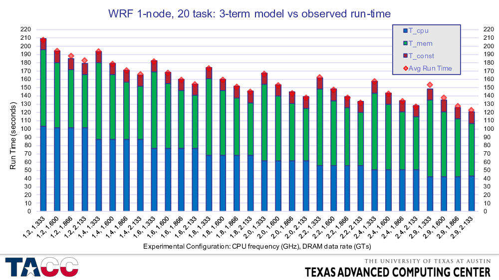
Bottom bars are model CPU time – easy to see the quantization.
Middle bars are model Memory time.
Top bars are (constant) IO time.
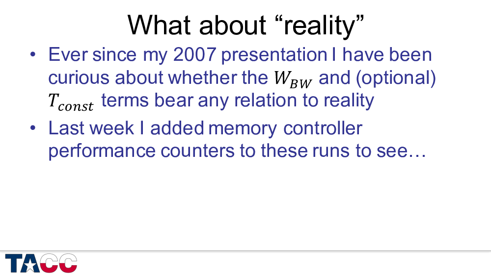
Drum roll, please….

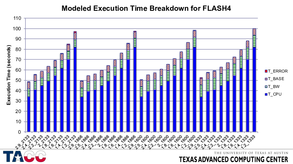
Ordered differently, but the same sort of picture.
Here the quantization of memory time is visible across the four groups of varying CPU frequencies.
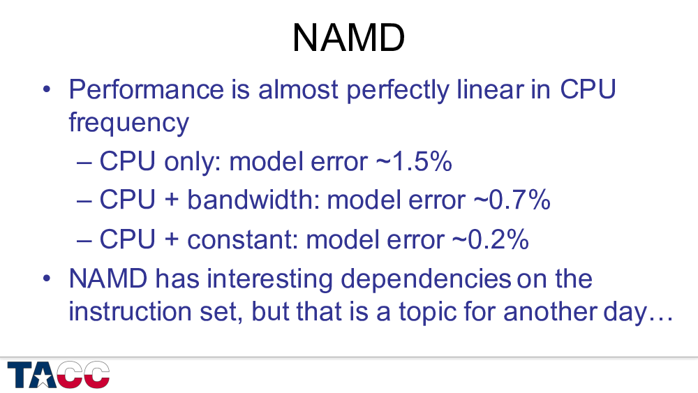
These NAMD results are not at all surprising — NAMD has extremely high cache re-use and therefore very low rates of main memory access — but it was important to see if this testing methodology replicated this expected result.
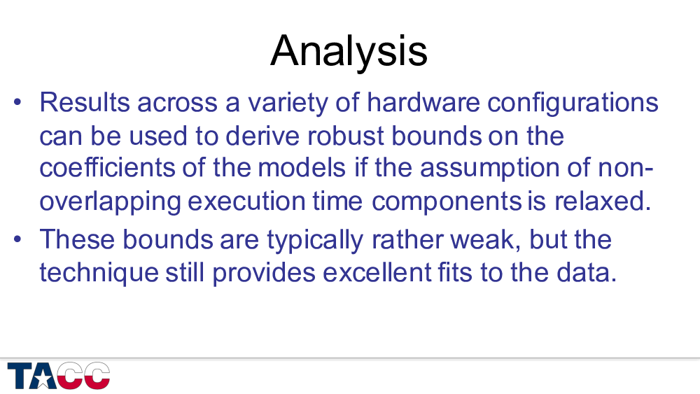
Big change of direction here….
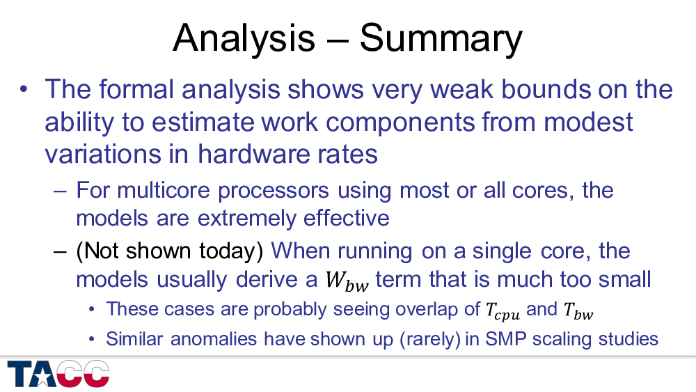
At the beginning I said that I was assuming that there would be no overlap across the execution times associated with the various work components.
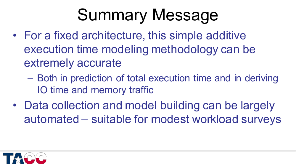
The extremely close agreement between the model results and observations strongly supports the effectiveness of this assumption.
On the other hand, overlap is certainly possible, so what can this methodology provide for us in the way of bounds on the degree of overlap?
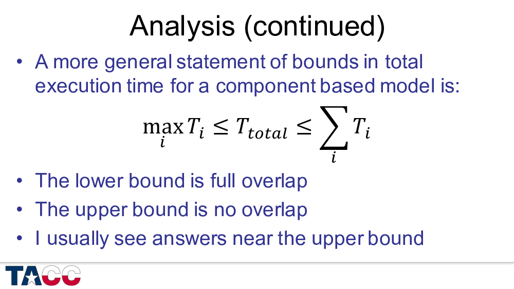
On some HW it is possible (but very rare) to get timings (slightly) outside these bounds – I ignore such cases here.
Note that maximum ratio of upper bound over lower bound is equal to “N” – the degrees of freedom of the model! This is an uncomfortably large range of uncertainty – making it even more important to understand bounds on overlap.
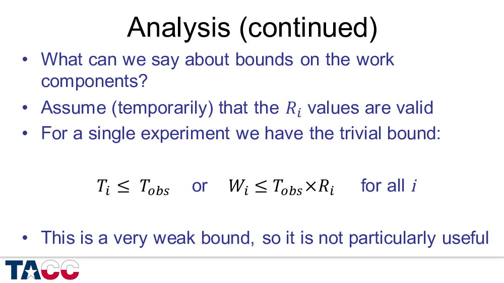
Physically this is saying that there can’t be so much work in any of the components that processing that work would exceed the total time observed.
But the goal is to learn something about the ratios of the work components, so we need to go further.
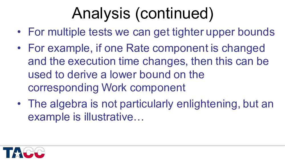
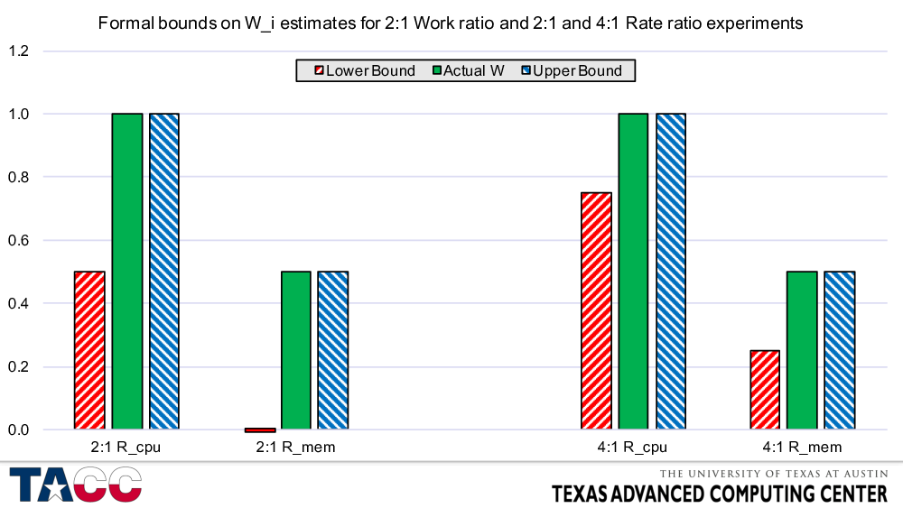
These numbers come from plugging in synthetic performance numbers from a model with variable overlap into the bounds analysis.
Message 1: If you want tight formal bounds on overlap, you need to be able to vary the “rate” parameters over a large range — probably too large to be practical.
Message 2: If one of the estimated time components is small and you cannot vary the corresponding rate parameter over a large enough range, it may be impossible to tell whether the work component is “fuller overlapped” or is associated with a negligible amount of work (e.g., the lower bound in the “2:1 R_mem” case in this figure). (See next slide.)
