
The Multicore Era
Over the past ~15 years, server processors from Intel and AMD have evolved from the early quad-core processors to the current monsters with over 50 cores per socket. The memory subsystems have grown at similar rates, from 3-4 DRAM channels at 1.333 GT/s transfer rates to 8-12 DRAM channels with 4.8 GT/s transfer rates, providing an aggregate peak memory bandwidth increase of 10x or more.
Sustainable memory bandwidth using multi-threaded code has closely followed the peak DRAM bandwidth, typically delivering best case throughput of 75%-85% of the peak DRAM bandwidth in each generation. Understanding sustained memory bandwidth in these systems starts with assuming 100% utilization and then reviewing the factors that get in the way (e.g., DRAM refresh, rank-to-rank stalls, read-to-write stalls, four-activate-window limitations, etc.).
What about single-core performance?
In my previous post, I reviewed historical data on single-core/single-thread memory bandwidth in multicore processors from Intel and AMD from 2010 to the present. The increase in single-core memory bandwidth has been rather slow overall, with Intel processors only showing about a 2x increase over the 13 years from 2010 to 2023.
Today I want to talk about what limits single-core bandwidth, and why the improvements in DRAM transfer rate and number of channels makes no difference for this case. This requires a completely different approach to modeling the memory system — one based on Little’s Law from queueing theory.
I was first introduced to Little’s Law by the late Burton Smith – probably in the late 1990’s. Little’s Law was developed in the context of queueing theory, where it relates the long-term average number of entries in a queue with their average arrival rate and their average wait time:
(Number of Entries in Queue) = (Arrival Rate) x (Average Waiting Time)
In the context of computer memory systems the same principles apply, but with different names:
Concurrency = Bandwidth x Latency
or with a bit more description:
(minimum required) Concurrency = (peak) Bandwidth * (minimum) Latency
Here:
- “Bandwidth” is the rate at which data is transferred from memory to the processor, with GB/s as the most convenient unit.
- “Latency” is the duration from the execution of a load instruction (to an address that misses in all the caches), and the completion of that load instruction when the data is returned from memory. Units of nanoseconds (ns) are most convenient.
- “Concurrency” is the amount of data that must be “in flight” between the core and the memory in order to maintain a steady-state system. From the form of the equation the units are GB/s * ns = Bytes, but to understand how this maps to computer hardware resources it is almost always more convenient to translate this to units of “cache lines” (with 64 Bytes per cache line in the processors reviewed here).
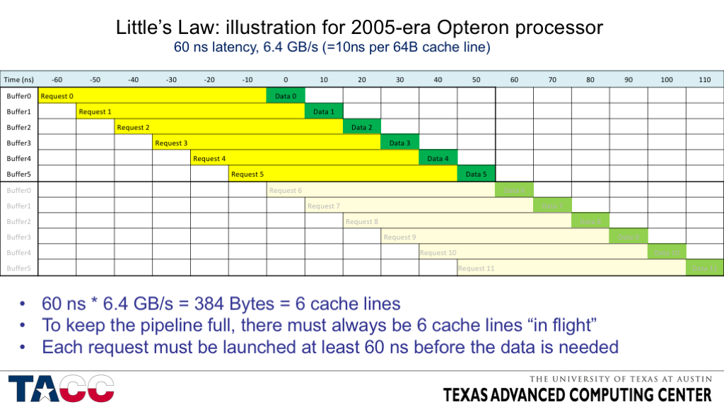
For recent systems the numerical values of concurrency are so large that they are difficult to show with modest-sized graphics. The example below is for a 2005-era processor with 60 ns memory latency and 6.4 GB/s peak DRAM bandwidth, requiring 6 concurrent 64-byte cache line accesses to be pending at all times to maintain full bandwidth. The processor supported 8 concurrent cache misses, so it was capable of satisfying the Little’s Law concurrency requirement using a single core.
A slightly different mental model:
Another way to think about Little’s Law is to replace the “bandwidth” term (GB/s) with a reciprocal term (usually called “gap”) having units of “ns/CacheLine”. For 64 Byte cache lines and the 32 GB/s peak bandwidth of the first example, this gives 2 ns/CacheLine. Substituting this alternate formation gives:
Concurrency (CacheLines) = Latency (ns) / Gap (ns/CacheLine)
This formulation suggests a different way of thinking about concurrency — supposed we have a latency of 64 ns and a transfer time per cache line of 2 ns. If we want to sustain full bandwidth, we need 64/2 =32 cache lines. We need to issue new read requests at the same (average) rate as data is received, so once every 2 ns. For the interface to be busy *now*, we needed to issue a read request (at least) 64 ns ago. For the interface to be busy immediately after the current transfer, we needed to issue a read request (at least) 62 ns ago. Ditto for 60, 58, 56, …, 2 ns in the past.
Computing required concurrency to get full bandwidth
Start with basic examples of computing the amount of concurrency needed to sustain full bandwidth in the presence of a known (minimum) latency:
- 2010 processor
- Xeon X5680, 6-core, “Westmere EP”
- 32 GB/s peak DRAM bandwidth (2 ns per cache line)
- 67 ns idle memory latency
- Required Concurrency: 32 GB/s * 67 ns = 2144 Bytes -> 33.5 cache lines -> 5.6 cache lines per core
- Available L1 cache miss concurrency: 10 cache lines per core
- 2023 processor:
- Xeon Max 9480, 56-core, “Sapphire Rapids”
- 307.2 GB/s peak DRAM bandwidth (0.2083 ns per cache line)
- 107 ns idle memory latency (configured in “flat mode” — one NUMA node per socket)
- Required Concurrency: 307.2 GB/s * 107 ns = 32870 Bytes -> 513 cache lines -> 9.2 cache lines per core
- Available L1 cache miss concurrency: 16 cache lines per core
In each of these examples, I used the peak memory bandwidth and the idle memory latency to compute the concurrency required to sustain full bandwidth. In both examples, using all the cores provides more than enough concurrency at the L1 Data Cache level to tolerate the memory latency and obtain full bandwidth (or close enough to “full” to run into other bandwidth limitations).
Computing upper bound on sustained bandwidth given limits on concurrency
The previous examples showed that one must use most of the cores to generate enough cache misses to fully tolerate the memory latency. What happens in the single-core case? Here we begin to see the flexibility and generality of Little’s Law. We simply rearrange to make “Bandwidth” the unknown, and compute it using the known concurrency and latency values.
(maximum sustained) Bandwidth <= (maximum available) Concurrency / (minimum possible) Latency
Important notes!
- “Bandwidth” here is not the peak bandwidth — it is an upper bound on the bandwidth that can be sustained.
- The “peak bandwidth” does not even occur in this equation — unless there is enough concurrency to tolerate the full latency, the sustained performance depends only on the concurrency and latency — not the peak bandwidth.
Using the same two example processors:
- 2010 processor, Xeon X5680:
- 10 64-Byte cache lines / 67 ns = 640 B / 67 ns = 9.55 GB/s
- 2023 processor: Xeon Max 9480:
- 16 64-Byte CacheLines / 107 ns = 1024 B / 107 ns = 9.57 GB/s
Are these reasonable upper bounds when compared to the measured single-core memory bandwidth?
Yes, but (on these Intel processors) only if the L2 hardware prefetchers are disabled.
- The L1 hardware prefetchers don’t matter here because they share the same set of cache miss tracking buffers as ordinary loads, so the maximum concurrency is unchanged. (The same is true for software prefetches.)
- There are more L2 cache miss handling buffers than L1 cache miss handling buffers, so using the L2 hardware prefetchers can increase the maximum concurrency.
With the L2 hardware prefetchers disabled, measured single-core read bandwidth never exceeds the upper bound. In most cases the measured bandwidth falls short of the bound. I can’t provide a demonstration of this assertion using these two example processors — the 2010-era Westmere processors are long gone and the new Xeon Max 9480 processors don’t allow me to fully disable the hardware prefetchers, but there are lots of other processors to play with.
For the Xeon Platinum 8280 (Cascade Lake) processors in the TACC Frontera system, the numbers are:
- Idle latency (ns) 68.s ns
- Max L1D misses 12 cache lines
- Measured single-core read BW 7.8 to 8.2 GB/s (2MiB to 2GiB array sizes with hardware prefetchers disabled)
- Upper Bound on single-core read BW 12 * 64 / 68.2 = 11.26 GB/s
- Shortfall ~25-30%
The bound is satisfied here, with the sustained single-core read bandwidth about 25%-30% less than the computed upper bound.
The discrepancy seems large. Fortunately recent Intel processors have a set of performance counters that can be used to take a closer look. For the L1D cache, the performance counter event L1D_PEND_MISS.PENDING increments every cycle by the number of pending L1D cache misses. This event can be modified with a threshold value, such that the counter only increments when the number of pending L1D cache misses meets or exceeds a specified threshold. When the threshold is set to 1, the event is called L1D_PEND_MISS.PENDING_CYCLES — the number of cycles that at least one L1D cache miss was pending. From these values and a count of the L1D cache misses, we can compute:
Average Number of L1D Misses = L1D_PEND_MISS.PENDING / L1D_PEND_MISS.PENDING_CYCLES
Average Duration of L1D Miss Buffer Occupancy = L1D_PEND_MISS.PENDING / Number_of_L1D_Misses
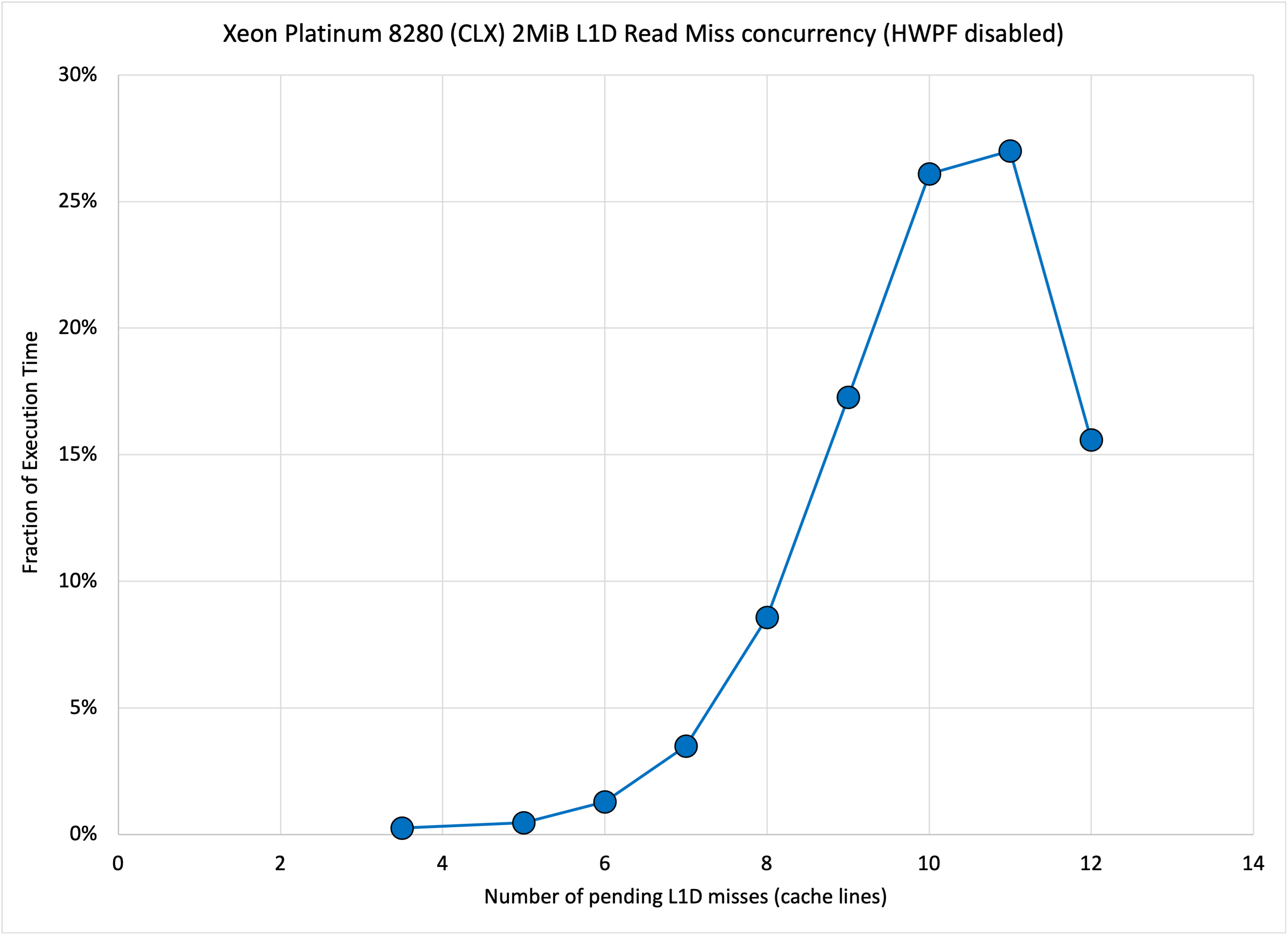
These counters were measured for the 2MiB read case (7.8 GB/s with HW Prefetchers disabled), giving:
- Average Number of L1D Misses: 10.04 <– 83.7% of the maximum (12 cache lines)
- Average Duration of L1D Miss Buffer Occupancy: 82.1 ns <– 20.4% higher than the idle latency (68.2 ns)
- Latency * BW = concurrency –> 82.1 * 7.8 = 640.4 Bytes = 10.01 cache lines
So the lines are accounted for, but the system does not sustain all 12 misses on average and for unknown reasons the L1D miss buffers are occupied for longer than initially expected.
By modifying the threshold value in the L1D_PEND_MISS.PENDING_CYCLES event, one can count the number of cycles at any desired minimum outstanding miss count. From these results the figure below shows the fraction of cycles with each miss count, showing that the maximum number of L1D misses only occurs in about 15% of cycles, with 10 or 11 misses in about 53% of the cycles.
I hope this brief introduction to Latency, Bandwidth, and Concurrency has been useful. Next time we will look at the impact of L2 hardware prefetchers on the Little’s Law interpretation of single-core memory bandwidth.